Summary

The context discusses the application of Kalman Filter for handling new observations in high-frequency data and its advantage over simple linear regression.

Abstract

The content of the context revolves around the implementation of the Kalman Filter in Python for dealing with streaming data, specifically high-frequency data. The author highlights the advantage of Kalman Filter over simple linear regression, as it allows for the quick update of the model with new observations without the need to include all past observations and recompute the regression. The context includes a Python code snippet demonstrating the implementation of the Kalman Filter class and its methods, including initialization, prediction, and update. The author also mentions the use of the Kalman Filter for cyclic datasets and the possibility of rewriting ARMA models in a state space form. The context concludes with an example of using the Kalman Filter on a resampled Yahoo SPY dataset, comparing it to AR(5) setup, and discussing the results.

Bullet points

The context discusses the application of Kalman Filter for handling new observations in high-frequency data.
The author highlights the advantage of Kalman Filter over simple linear regression in dealing with new observations.
The context includes a Python code snippet demonstrating the implementation of the Kalman Filter class and its methods.
The author mentions the use of the Kalman Filter for cyclic datasets and the possibility of rewriting ARMA models in a state space form.
The context concludes with an example of using the Kalman Filter on a resampled Yahoo SPY dataset, comparing it to AR(5) setup, and discussing the results.

Timeseries Methods: Kalman Filter from scratch in Python — Part 2

In Part 1 we talked about applying simple Kalman Filter, the advantage of Kalman Filter lies in its ability to deal with new observation （streaming data). This is a huge advantage when dealing with high frequency data. If the model is simple there is no need to include all past observation and recompute the simple linear regression.

class kalman_filter:
    def __init__(self, x_init, F, Q, R, H, B=None, u=None, sd=np.array([[0]])):
        self.x_init = x_init
        self.F = F
        self.Q = Q
        self.R = R
        self.H = H
        self.X_post = self.x_init
        self.P_post = sd
        self.X_prior = None
        self.P_prior = None
        if B is not None and u is not None:
            self.B = B
            self.u = u
        else:
            self.B = np.array([[0]])
            self.u = np.array([[0]])

        self.mean = np.array([[]])
        self.covar = np.array([[]])

    def fit(self, data, num_state=1, fit_step=None):
        self.num_state = num_state
        fit_step = fit_step if fit_step is not None and fit_step < data.shape[1] else data.shape[1]
        for i in range(fit_step):
            z_k = data[:, i]
            # predict
            self._predict(self.X_post, self.P_post)
            self._update(z_k)
            # update
            self.mean = np.append(self.mean, self.X_post)
            self.covar = np.append(self.covar, self.P_post)

    def _predict(self, X_post, P_post):
        self.X_prior = np.dot(self.F, X_post) + np.dot(self.B, self.u)
        self.X_prior = self.X_prior.reshape(X_post.shape)
        self.P_prior = np.dot(np.dot(self.F, P_post), self.F.T) + self.Q

    def _update(self, observation):
        resid = observation - np.dot(self.H, self.X_prior)
        S_k = np.dot(np.dot(self.H, self.P_prior), self.H.T) + self.R
        K_k = np.dot(np.dot(self.P_prior, self.H.T), np.linalg.inv(S_k))
        self.X_post = self.X_prior + np.dot(K_k, resid)
        self.P_post = np.dot(np.eye(self.num_state) - np.dot(K_k, self.H), self.P_prior)

    def new_observation(self, observation):
        num_new_obs = observation.shape(self.num_state)
        for i in range(num_new_obs):
            obs = observation[:,i]
            self._predict(self.X_post, self.P_post)
            self._update(self, obs)

From the above code break we can see that with new observation, we only really need the X and P posterior from the earlier to quickly update.

Whereas for regular regression when there is a new observation, we generally would rerun the fit to include history and the new observation. It is not as trivial to only use past fitting result and update it with the new dataset.

Simple linear regression may not be suitable for cyclic dataset. Given that we can easily rewrite ARMA model in a state space form. There are multiple ways to include season adjustment when applying kalman filter. One can easily found proofs online, check this link for more details.

Using the same dataset as previous post (Yahoo, SPY). To make it simpler we update the timeseries such that there is a datapoint for each weekday （regardless of holiday or not）, and that holiday will be filled with previous business day value. For a detailed list of resampling rule in python, please see the documentation here.

data = data.resample('B').ffill()

To simplify the code, all evaluations will be done using available python packages (pykalman for kalman and statsmodels for ARMA).

    
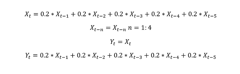
#setup 1
n_season = 5
F = np.zeros((n_season, n_season))
F[0,:] = [0.2] * 5
F[1:,:-1] = np.eye(n_season - 1)
H = np.array([1,0,0,0,0])

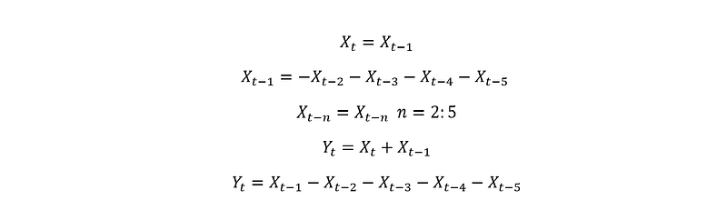
#setup 2
F[0,0] = 1
F[1, 1:-1] = [-1.0] * (n_season - 1)
F[2:,1:-1] = np.eye(n_season - 1)
H = np.array([1, 1, 0, 0, 0, 0])
P_init = np.eye(n_season + 1) * 0
P_init[:2,:2] = np.eye(1) * Q

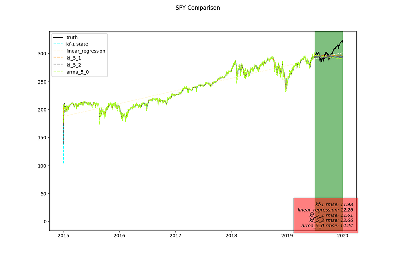
These setups are compared against the two models in previous post as well as the standard AR(5) setup. Below are the results. The RMSE is computed on the test dataset only.

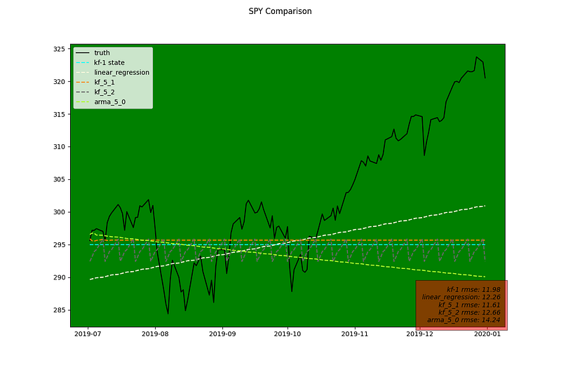
Magnify the testing region we notice that for the 5 state KF model as time horizon extends further into the future it becomes a straight prediction. The alternative setup ensures that seasonality trend is preserved.

This is because if we expand the matrix, we have the following equations:

The interpretation is pretty straight forward from the two setups above. Which choice is better is dependent on the dataset. Both of these are simple models and ideally, we would prefer to stack them together to produce a better model. As explained in this article, a group of weak learners is preferred over one complex learner. We will also explore options to stack weak learners in future posts.