avatarBenjamin Obi Tayo Ph.D.

Free AI web copilot to create summaries, insights and extended knowledge, download it at here

3115

Abstract

igure id="e909"><img src="https://cdn-images-1.readmedium.com/v2/resize:fit:800/1*wNd_J9lYsAG4dn2Gq6FJIg.png"><figcaption></figcaption></figure><p id="746a">This matrix can be diagonalized by performing a unitary transformation (PCA transformation) to obtain the following:</p><figure id="8b7f"><img src="https://cdn-images-1.readmedium.com/v2/resize:fit:800/1*YSgemfsENV7hRp0bm8Mnug.png"><figcaption></figcaption></figure><p id="a927">Since the trace of a matrix remains invariant under a unitary transformation, we observe that the sum of the eigenvalues of the diagonal matrix is equal to the total variance contained in features X1, X2, X3, and X4. Hence, we can define the following quantities:</p><figure id="06a9"><img src="https://cdn-images-1.readmedium.com/v2/resize:fit:800/1*xf-yYARQye5pzpAQePx6PQ.png"><figcaption></figcaption></figure><p id="843e">Notice that when p = 4, the cumulative variance becomes equal to 1 as expected.</p><h1 id="7a3c">III. R Implementation of PCA</h1><p id="5588">To illustrate how PCA works, we show an example by examining the iris dataset. The R code can be downloaded from here: <a href="https://github.com/bot13956/principal_component_analysis_iris_dataset/blob/master/PCA_irisdataset.R"><i>https://github.com/bot13956/principal_component_analysis_iris_dataset/blob/master/PCA_irisdataset.R</i></a></p><p id="e610">Let us look at the covariance matrix:</p><figure id="69e5"><img src="https://cdn-images-1.readmedium.com/v2/resize:fit:800/0*4lPMl0eIcKdeCMOa.png"><figcaption><b>Table 2</b>. Correlation matrix for the iris dataset.</figcaption></figure><p id="0716"><b>Table 2</b> shows strong correlations between original features in the iris dataset. <b>Figure 2</b> is a pairplot that shows scatter plots, density plots, and correlation coefficients between original features. Notice the strong correlations between original features.</p><figure id="afa4"><img src="https://cdn-images-1.readmedium.com/v2/resize:fit:800/0*c5OfKq-kEQovQK5t.png"><figcaption><b>Figure 2</b>. Pairplot for iris dataset in original feature space.</figcaption></figure><p id="3cf8">Let us now examine the transformed covariance matrix:</p><figure id="edd7"><img src="https://cdn-images-1.readmedium.com/v2/resize:fit:800/0*DA-m_PQf5ll745sd.png"><figcaption><b>Table 3</b>. Covariance matrix in PCA space.</figcaption></figure><p id="a7a7"><b>Table 3</b> shows zero correlations between transformed features. <b>Figure 4</b> shows the pairplot in the PCA space. We see that the correlation between features has been removed.</p><figure id="cd44"><img src="https://cdn-images-1.readmedium.com/v2/resize:fit:800/0*IfTfXii83d1C7qJD.png"><figcaption><b>Figure 3</b>. Pairplot for iris dataset in PCA space.</figcaption></figure><p id="4e56"><b>Table 4</b> contains a summary of helpful indicators from a PCA calculation:</p><figure id="0a8d"><img src="https://cdn-images-1.readmedium.com/v2/resize:fit:800/0*i1u5iDWYstJgilf_.png"><figcaption><b>Table 4</b>. Summary of useful indicators from PCA calculation.</figcaption></figure><p id="f548">Based on this summary, we see that 99.5 percent of

Options

the variance is contributed by the first three principal components (p = 3). This means that in the final model, the fourth principal component PC4 could be dropped since its contribution to the variance is negligible.</p><h1 id="f1d4">IV. Summary and Conclusion</h1><p id="3b4d">In summary, we’ve explained the mathematical foundations of PCA and we showed how the PCA algorithm can be implemented in R using the iris dataset for illustrative purposes. The R code used for performing the calculations can be downloaded from here: <a href="https://github.com/bot13956/principal_component_analysis_iris_dataset/blob/master/PCA_irisdataset.R"><i>https://github.com/bot13956/principal_component_analysis_iris_dataset/blob/master/PCA_irisdataset.R</i></a></p><h1 id="cb8d">Additional Data Science/Machine Learning Resources</h1><p id="adfb"><a href="https://towardsdatascience.com/data-science-minimum-10-essential-skills-you-need-to-know-to-start-doing-data-science-e5a5a9be5991">Data Science Minimum: 10 Essential Skills You Need to Know to Start Doing Data Science</a></p><p id="369a"><a href="https://readmedium.com/data-science-curriculum-bf3bb6805576">Data Science Curriculum</a></p><p id="65e0"><a href="https://readmedium.com/4-math-skills-for-machine-learning-12bfbc959c92">Essential Maths Skills for Machine Learning</a></p><p id="7617"><a href="https://readmedium.com/3-best-data-science-mooc-specializations-d58da382f628">3 Best Data Science MOOC Specializations</a></p><p id="1eae"><a href="https://towardsdatascience.com/5-best-degrees-for-getting-into-data-science-c3eb067883b1">5 Best Degrees for Getting into Data Science</a></p><p id="6dbc"><a href="https://towardsdatascience.com/5-reasons-why-you-should-begin-your-data-science-journey-in-2020-2b4a0a5e4239">5 reasons why you should begin your data science journey in 2020</a></p><p id="06ff"><a href="https://towardsdatascience.com/theoretical-foundations-of-data-science-should-i-care-or-simply-focus-on-hands-on-skills-c53fb0caba66">Theoretical Foundations of Data Science — Should I Care or Simply Focus on Hands-on Skills?</a></p><p id="ada8"><a href="https://towardsdatascience.com/machine-learning-project-planning-71bdb3a44349">Machine Learning Project Planning</a></p><p id="ca19"><a href="https://towardsdatascience.com/how-to-organize-your-data-science-project-dd6599cf000a">How to Organize Your Data Science Project</a></p><p id="e8b7"><a href="https://readmedium.com/productivity-tools-for-large-scale-data-science-projects-64810dfbb971">Productivity Tools for Large-scale Data Science Projects</a></p><p id="db8f"><a href="https://towardsdatascience.com/a-data-science-portfolio-is-more-valuable-than-a-resume-2d031d6ce518">A Data Science Portfolio is More Valuable than a Resume</a></p><p id="a082"><a href="https://readmedium.com/data-science-101-a-short-course-on-medium-platform-with-r-and-python-code-included-3cdc9d489c6d">Data Science 101 — A Short Course on Medium Platform with R and Python Code Included</a></p><p id="8859"><b><i>For questions and inquiries, please email me</i></b>: [email protected]</p></article></body>

Image by Benjamin O. Tayo

Data Science

Mathematics of Principal Component Analysis with R Code Implementation

Theoretical foundations of principal component analysis (PCA) with R code implementation

I. Introduction

In machine learning, a dataset containing features (predictors) and discrete class labels (for a classification problem such as logistic regression); or features and continuous outcomes (for a linear regression problem), is used to build a predictive model that can make predictions on unseen data. The predictive power of a model depends greatly on the quality and size of the training dataset.

Generally, the larger the dataset the better, however, there is a tradeoff between the size of the dataset and computational time needed for training. It turns out that in very large datasets, there might be lots of redundancy in the features or lots of unimportant features in the dataset, and hence dimensionality reduction techniques could be used for selecting only a limited number of relevant features needed for training.

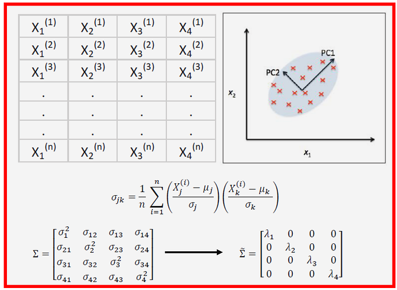
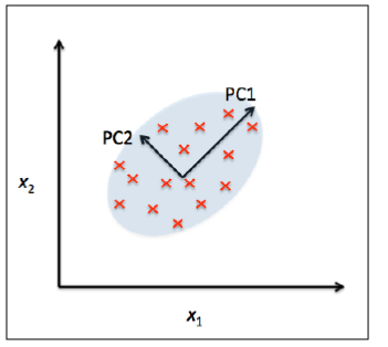
Principal Component Analysis (PCA) is a statistical method that is used for feature extraction. PCA is used for high-dimensional and highly correlated data. The basic idea of PCA is to transform the original space of features into the space of principal components, as shown in Figure 1 below:

Figure 1: PCA algorithm transforms from old to new feature space so as to remove feature correlation. Image by Benjamin O. Tayo

A PCA transformation achieves the following:

a) Reduce the number of features to be used in the final model by focusing only on the components accounting for the majority of the variance in the dataset.

b) Removes the correlation between features.

II. Mathematical Basis of PCA

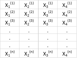
Suppose we have a highly correlated features matrix with 4 features and n observation as shown in Table 1 below:

Table 1. Features matrix with 4 variables and n observations.

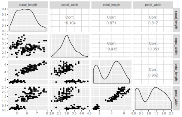
To visualize the correlations between the features, we can generate a scatter plot, as shown in Figure 1. To quantify the degree of correlation between features, we can compute the covariance matrix using this equation:

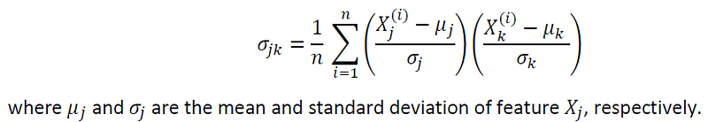
In matrix form, the covariance matrix can be expressed as a 4 x 4 symmetric matrix:

This matrix can be diagonalized by performing a unitary transformation (PCA transformation) to obtain the following:

Since the trace of a matrix remains invariant under a unitary transformation, we observe that the sum of the eigenvalues of the diagonal matrix is equal to the total variance contained in features X1, X2, X3, and X4. Hence, we can define the following quantities:

Notice that when p = 4, the cumulative variance becomes equal to 1 as expected.

III. R Implementation of PCA

To illustrate how PCA works, we show an example by examining the iris dataset. The R code can be downloaded from here: https://github.com/bot13956/principal_component_analysis_iris_dataset/blob/master/PCA_irisdataset.R

Let us look at the covariance matrix:

Table 2. Correlation matrix for the iris dataset.

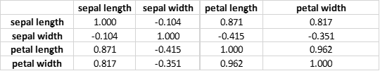
Table 2 shows strong correlations between original features in the iris dataset. Figure 2 is a pairplot that shows scatter plots, density plots, and correlation coefficients between original features. Notice the strong correlations between original features.

Figure 2. Pairplot for iris dataset in original feature space.

Let us now examine the transformed covariance matrix:

Table 3. Covariance matrix in PCA space.

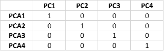
Table 3 shows zero correlations between transformed features. Figure 4 shows the pairplot in the PCA space. We see that the correlation between features has been removed.

Figure 3. Pairplot for iris dataset in PCA space.

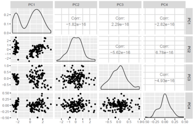
Table 4 contains a summary of helpful indicators from a PCA calculation:

Table 4. Summary of useful indicators from PCA calculation.

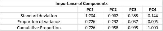
Based on this summary, we see that 99.5 percent of the variance is contributed by the first three principal components (p = 3). This means that in the final model, the fourth principal component PC4 could be dropped since its contribution to the variance is negligible.

IV. Summary and Conclusion

In summary, we’ve explained the mathematical foundations of PCA and we showed how the PCA algorithm can be implemented in R using the iris dataset for illustrative purposes. The R code used for performing the calculations can be downloaded from here: https://github.com/bot13956/principal_component_analysis_iris_dataset/blob/master/PCA_irisdataset.R

Additional Data Science/Machine Learning Resources

Data Science Minimum: 10 Essential Skills You Need to Know to Start Doing Data Science

Data Science Curriculum

Essential Maths Skills for Machine Learning

3 Best Data Science MOOC Specializations

5 Best Degrees for Getting into Data Science

5 reasons why you should begin your data science journey in 2020

Theoretical Foundations of Data Science — Should I Care or Simply Focus on Hands-on Skills?

Machine Learning Project Planning

How to Organize Your Data Science Project

Productivity Tools for Large-scale Data Science Projects

A Data Science Portfolio is More Valuable than a Resume

Data Science 101 — A Short Course on Medium Platform with R and Python Code Included

For questions and inquiries, please email me: [email protected]

Data Science
Machine Learning
Feature Engineering
Dimensionality Reduction
Iris Dataset
Recommended from ReadMedium