LLM Architectures Explained: Transformers (Part 6)

Deep Dive into the architecture & building real-world applications leveraging NLP Models starting from RNN to Transformer.

Posts in this Series

1. NLP Fundamentals
2. Word Embeddings
3. RNNs, LSTMs & GRUs
4. Encoder-Decoder Architecture
5. Attention Mechanism
6. Transformers ( This Post )
7. Coding a Transformer
8. BERT
9. GPT
10. LLama
11. Mistral

Table of Contents

· 1. Introduction ∘ 1.1 How are LLMs built and trained? ∘ 1.2 Background: The Pre-Transformer Era ∘ 1.3 Introducing Transformers ∘ 1.4 Why “Attention is All You Need”? · 2. Transformer Architecture · 2.1 Embedding ∘ 2.1.1 Input Embedding · 2.2 The Encoder ∘ 2.2.1 Multi-Headed Self-Attention ∘ 2.2.2 Normalization and Residual Connections ∘ 2.2.3 Feed-Forward Neural Network ∘ 2.2.4 Output of the Encoder · 2.3 The Decoder ∘ 2.3.1 Output Embeddings ∘ 2.3.2 Positional Encoding ∘ 2.3.3 Stack of Decoder Layers ∘ 2.3.4 Linear Classifier and Softmax for Generating Output Probabilities ∘ 2.3.5 Normalization and Residual Connections ∘ 2.3.6 Output of the Decoder · 3. LLM Architectures ∘ 3.1 Seq-2-Seq Models (Encoder-decoder) ∘ 3.2 AutoEncoding Models (Encoder-only) ∘ 3.3 AutoRegressive Models (Decoder-only) ∘ 3.4 Mixture of Experts (MoE) · 4. Inference ∘ 4.1 Inference Techniques ∘ 4.1.1 Greedy Search ∘ 4.1.2 Beam Search · 5. Transformer Inference Optimization ∘ 5.1 Transformer Architecture and Inference Flow ∘ 5.2 Phases of Transformer Inference: Prefill and Decode · 6. Challenges in Transformer Inference · 7. Optimization Techniques for Faster Inference ∘ 7.1 Quantization ∘ 7.2 Key-Value (KV) Caching ∘ 7.3 Speculative Decoding ∘ 7.4 Batching ∘ 7.5 Hardware Optimisation: Parallelism ∘ 7.6 FlashAttention and Memory Efficiency · 8. Benchmarking Inference Performance ∘ 8.1 Trends in Transformer Inference ∘ 8.1.1 Memory Optimization with Paging and FlashAttention ∘ 8.1.2 Multi-Query and Grouped-Query Attention ∘ 8.1.3 Parallelism: Tensor and Sequence ∘ 8.1.4. Speculative Inference for Real-Time Applications · 9. Handling Large Datasets ∘ 9.1 Efficient Data Loading and Preprocessing ∘ 9.2 Distributed Training ∘ 9.3 Mixed Precision Training ∘ 9.4 Gradient Accumulation ∘ 9.5 Checkpointing and Resuming ∘ 9.6 Data Augmentation and Sampling · 10. Conclusion · 11. Test your Knowledge! ∘ 11.1 DIY

1. Introduction

A Large Language Model (LLM) is a type of artificial intelligence (AI) algorithm that uses deep learning techniques and massive data sets to achieve general-purpose language understanding and generation. LLMs are pre-trained on vast amounts of data, often including sources like the Common Crawl and Wikipedia.

LLMs are designed to recognize, summarize, translate, predict, and generate text and other forms of content based on the knowledge gained from their training.

Key characteristics of LLMs include:

• Transformer Model Architecture — LLMs are based on transformer models, which consist of an encoder and a decoder that extract meanings from a sequence of text and understand the relationships between words.
• Attention Mechanism — This mechanism allows LLMs to capture long-range dependencies between words, enabling them to understand context.
• Autoregressive Text Generation — LLMs generate text based on previously generated tokens, allowing them to produce text in different styles and languages.

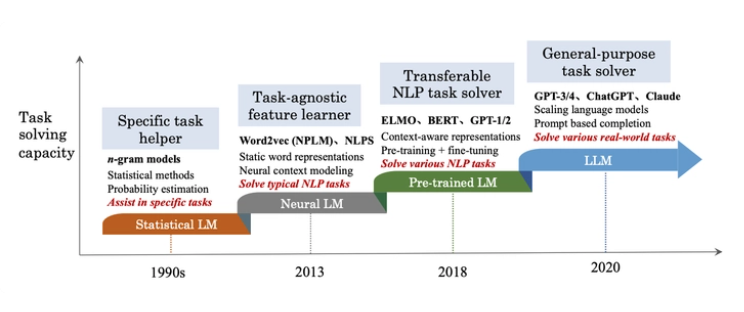
Some popular examples of LLMs are GPT-3 and GPT-4 from OpenAI, LLaMA 2 from Meta, and Gemini from Google. These models have the potential to disrupt various industries, including search engines, natural language processing, healthcare, robotics, and code generation.

1.1 How are LLMs built and trained?

Building and training Large Language Models (LLMs) is a complex process that involves several steps. Initially, a massive amount of text data is collected from various sources such as books, websites, and social media posts. This data is then cleaned and processed into a format that the AI can learn from.

The architecture of the LLMs is designed using deep neural networks with billions of parameters. Different transformer architectures like encoder-decoder, causal decoder, and prefix decoder are used, and the design of the model significantly impacts its capabilities.

The LLMs are then trained using computational power and optimization algorithms. This training tunes the parameters to predict text statistically, and more training leads to more capable models.

Finally, by scaling up data, parameters, and compute power, companies have been able to produce LLMs with capabilities approaching human language use.

• Data Collection — LLMs require huge datasets of text data to train on. This can include books, websites, social media posts, and more. Data is cleaned and processed into a format the AI can learn from.
• Model Architecture — LLMs have a deep neural network architecture with billions of parameters. Different architectures like Transformer or GPT are used. The model design impacts its capabilities.
• Training — LLMs are trained using computational power and optimization algorithms. Training tunes the parameters to predict text statistically. More training leads to more capable models.
• Scaling — By scaling up data, parameters, and compute power, companies have produced LLMs with capabilities approaching human language use.

Large Language Model Operations (LLMOps) concentrates on the effective deployment, monitoring, and upkeep of LLMs in production. It encompasses model versioning, scaling, and performance enhancement.

1.2 Background: The Pre-Transformer Era

Transformers were developed to solve the problem of sequence transduction, or neural machine translation. That means any task that transforms an input sequence to an output sequence. This includes speech recognition, text-to-speech transformation, etc.

For sequence transduction models to work effectively, memory is essential. For example, when translating the sentence:

“The Transformers are a Japanese hardcore punk band. The band was formed in 1968 during the height of Japanese music history”

the phrase “the band” refers back to “The Transformers.” Recognizing these connections is crucial for accurate translation. Models like Recurrent Neural Networks (RNNs) and Convolutional Neural Networks (CNNs) have traditionally addressed these dependencies, but both have limitations. Let’s quickly explore these architectures and their drawbacks.

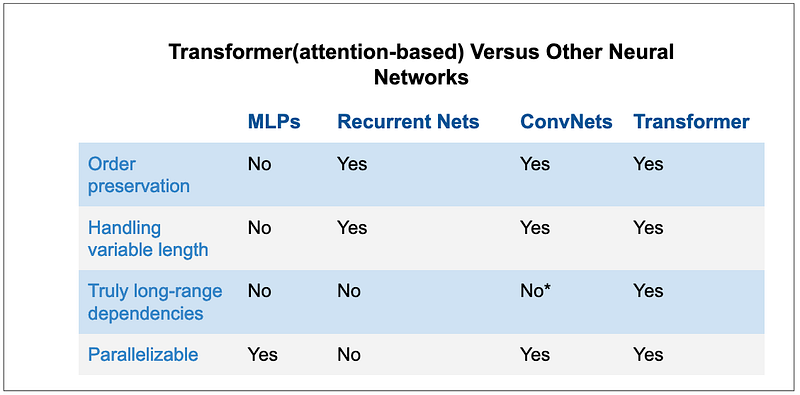
1.2.1 MultiLayer Perceptrons (MLPs)

Let’s start with multilayer perceptrons (MLPs), one of the classical neural network approaches. MLPs are not super powerful themselves but you will find them integrated in almost any other architecture(surprisingly even in transformer). MLPs are basically a sequence of linear layers or fully connected layers.

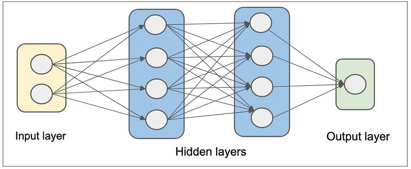
MLPs have long been used to model different kinds of data way before the AI community find best architectures for various modalities but one thing for sure, they are not suitable for sequence modelling. Due to their feedforward design, they can not preserve the order of information in a sequence. Sequence data lose meaning when the order of the data is lost. Thus, the inability of MLPs to preserve order of information make them unsuitable for sequence modelling. Also, MLPs takes lots of paramaters which is another undesired property a neural network can have.

1.2.2 Recurrent Neural Networks (RNNs)

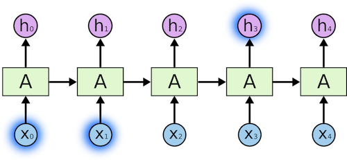
Recurrent Neural Networks have loops in them, allowing information to persist.

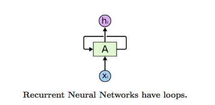
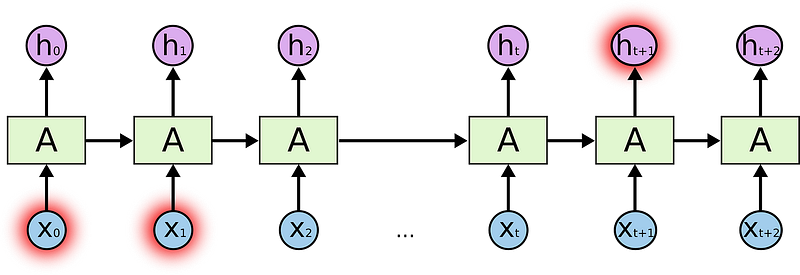
In the above diagram, a chunk of neural network, A, looks at some input xt and outputs a value ht. A loop allows information to be passed from one step of the network to the next. A recurrent neural network can be thought of as multiple copies of the same network, each passing a message to a successor. Consider what happens if we unroll the loop:

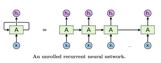
This chain-like nature reveals that recurrent neural networks are intimately related to sequences and lists. They’re the natural architecture of neural network to use for such data. And they certainly are used! In the last few years, there have been incredible success applying RNNs to a variety of problems: speech recognition, language modeling, translation, image captioning… The list goes on.

The following picture shows how usually a sequence to sequence model works using RNNs. Each word is processed separately, and the resulting sentence is generated by passing a hidden state to the decoding stage that, then, generates the output.

The problem of long-term dependencies

Consider a language model that is trying to predict the next word based on the previous ones. If we are trying to predict the next word of the sentence “the clouds in the ….”, we don’t need further context. It’s pretty obvious that the next word is going to be sky.

In this case where the difference between the relevant information and the place that is needed is small, RNNs can learn to use past information and figure out what is the next word for this sentence.

But there are cases where we need more context. For example, let’s say that you are trying to predict the last word of the text: “I grew up in France… I speak fluent …”. Recent information suggests that the next word is probably a language, but if we want to narrow down which language, we need context of France, that is further back in the text.

RNNs become very ineffective when the gap between the relevant information and the point where it is needed become very large. That is due to the fact that the information is passed at each step and the longer the chain is, the more probable the information is lost along the chain.

So, what are RNNs’ main problems? They are quite ineffective for NLP tasks for two main reasons:

• They process the input data sequentially, one after the other. Such a recurrent process does not make use of modern graphics processing units (GPUs), which were designed for parallel computation and, thus, makes the training of such models quite slow.
• They become quite ineffective when elements are distant from one another. This is due to the fact that information is passed at each step and the longer the chain is, the more probable the information is lost along the chain.

1.2.3 Long Short-Term Memory (LSTM)

When arranging one’s calendar for the day, we prioritize our appointments. If there is anything important, we can cancel some of the meetings and accommodate what is important.

RNNs don’t do that. Whenever it adds new information, it transforms existing information completely by applying a function. The entire information is modified, and there is no consideration of what is important and what is not.

LSTMs make small modifications to the information by multiplications and additions. With LSTMs, the information flows through a mechanism known as cell states. In this way, LSTMs can selectively remember or forget things that are important and not so important.

Internally, a LSTM looks like the following:

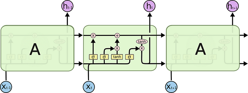
Each cell takes as inputs x_t (a word in the case of a sentence to sentence translation), the previous cell state and the output of the previous cell. It manipulates these inputs and based on them, it generates a new cell state, and an output. I won’t go into detail on the mechanics of each cell. If you want to understand how each cell works, I recommend Christopher’s blog post:

With a cell state, the information in a sentence that is important for translating a word may be passed from one word to another, when translating.

The problem with LSTMs

The same problem that happens to RNNs generally, happen with LSTMs, i.e. when sentences are too long LSTMs still don’t do too well. The reason for that is that the probability of keeping the context from a word that is far away from the current word being processed decreases exponentially with the distance from it.

That means that when sentences are long, the model often forgets the content of distant positions in the sequence. Another problem with RNNs, and LSTMs, is that it’s hard to parallelize the work for processing sentences, since you are have to process word by word. Not only that but there is no model of long and short range dependencies.

To summarize, LSTMs and RNNs present 3 problems:

• Sequential computation inhibits parallelization
• No explicit modeling of long and short range dependencies
• “Distance” between positions is linear

1.2.4 Attention Mechanism

To solve some of these problems, researchers created a technique for paying attention to specific words.

When translating a sentence, I pay special attention to the word I’m presently translating. When I’m transcribing an audio recording, I listen carefully to the segment I’m actively writing down. And if you ask me to describe the room I’m sitting in, I’ll glance around at the objects I’m describing as I do so.

Neural networks can achieve this same behavior using attention, focusing on part of a subset of the information they are given. For example, an RNN can attend over the output of another RNN. At every time step, it focuses on different positions in the other RNN.

To solve these problems, Attention is a technique that is used in a neural network. For RNNs, instead of only encoding the whole sentence in a hidden state, each word has a corresponding hidden state that is passed all the way to the decoding stage. Then, the hidden states are used at each step of the RNN to decode. The following gif shows how that happens.

The idea behind it is that there might be relevant information in every word in a sentence. So for the decoding to be precise, it needs to take into account every word of the input, using attention.

For attention to be brought to RNNs in sequence transduction, we divide the encoding and decoding into 2 main steps. One step is represented in green and the other in purple. The green step is called the encoding stage and the purple step is the decoding stage.

The step in green in charge of creating the hidden states from the input. Instead of passing only one hidden state to the decoders as we did before using attention, we pass all the hidden states generated by every “word” of the sentence to the decoding stage. Each hidden state is used in the decoding stage, to figure out where the network should pay attention to.

For example, when translating the sentence “Je suis étudiant” to English, requires that the decoding step looks at different words when translating it.

This gif shows how the weight that is given to each hidden state when translating the sentence “Je suis étudiant” into English. The darker the color is, the more weight is associated with each word.

But some of the problems that we discussed, still are not solved with RNNs using attention. For example, processing inputs (words) in parallel is not possible. For a large corpus of text, this increases the time spent translating the text.

Drawbacks of the Attention Mechanism:

Sequential Training: The traditional Encoder-Decoder architecture, which is LSTM-based, processes one word at a time, making training inherently sequential. This limits parallelism during training, resulting in slower training times. Due to the sequential nature, scaling to large datasets becomes inefficient, making transfer learning impractical.

As a result, models cannot be fine-tuned efficiently, forcing training from scratch for each task. This leads to higher computational costs, longer training times, and increased data requirements, significantly raising the cost of each training cycle.

1.2.5 Convolutional Neural Networks (CNNs)

Convolutional Neural Networks (CNNs) offer significant advantages when addressing sequence transduction tasks:

• Parallelism: CNNs are easily parallelized at the layer level, meaning multiple parts of the input can be processed simultaneously, resulting in faster computation compared to sequential models like RNNs.
• Local Dependency Exploitation: CNNs excel at capturing local patterns and relationships between nearby elements (such as words in a sentence) through convolutional filters, which focus on smaller regions of the input data.
• Logarithmic Distance: In CNNs, the “distance” between any input and output element is logarithmic in terms of the number of layers (log(N)). This means the number of operations required to connect distant elements is significantly reduced compared to RNNs, where the distance between elements grows linearly with sequence length (N).

Some of the most widely known sequence transduction models, such as WaveNet and ByteNet, are built on CNN architectures. In models like WaveNet, each input (word or token) is processed independently of the previous one, enabling parallel processing. This means that CNNs avoid the sequential bottleneck of RNNs, where each word is dependent on the previous one.

Additionally, in CNNs, the “distance” between the output and any input is proportional to the depth of the network, roughly log(N). This is significantly more efficient than RNNs, where the distance grows linearly (N), making CNNs faster for sequence processing.

However, CNNs have a limitation in handling long-range dependencies. They struggle to effectively model relationships between distant words in a sequence, especially when context from far-apart tokens is critical. This is why Transformers were introduced — they combine the parallelism of CNNs with the self-attention mechanism, which captures both local and global dependencies efficiently.

1.3 Introducing Transformers

To solve the problem of parallelization, Transformers try to solve the problem by using encoders and decoders together with attention models. Attention boosts the speed of how fast the model can translate from one sequence to another.

Let’s take a look at how Transformer works. Transformer is a model that uses attention to boost the speed. More specifically, it uses self-attention.

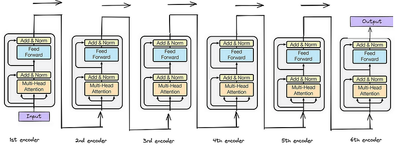
Internally, the Transformer has a similar kind of architecture as the previous models above. But the Transformer consists of six encoders and six decoders.

There are three seminal papers that laid the foundation for Transformer models:

1. Sequence to Sequence Learning with Neural Networks 2. Neural Machine Translation by Jointly Learning to Align and Translate 3. Attention is All You Need

1.4 Why “Attention is All You Need”?

1. Replacement of LSTM with Self-Attention: The introduction of self-attention in place of LSTM-based architectures enabled parallelized training, significantly speeding up the training process. 2. Stable Architecture: The Transformer architecture became robust by combining several smaller components, such as positional encoding and multi-head attention, leading to a scalable and reliable model design.

3. Stable Hyperparameters: The hyperparameters used in the original Transformer architecture have proven to be stable and resilient over time. Remarkably, many Transformer-based models today still use similar hyperparameter values, demonstrating their robustness across various tasks and datasets.

Let’s look into the Transformer architecture in detail.

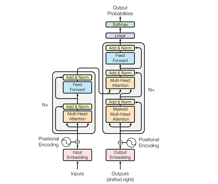
2. Transformer Architecture

Fundamentally, text-generative Transformer models operate on the principle of next-word prediction: given a text prompt from the user, what is the most probable next word that will follow this input? The core innovation and power of Transformers lie in their use of self-attention mechanism, which allows them to process entire sequences and capture long-range dependencies more effectively than previous architectures.

Originally devised for sequence transduction or neural machine translation, transformers excel in converting input sequences into output sequences. It is the first transduction model relying entirely on self-attention to compute representations of its input and output without using sequence-aligned RNNs or convolution. The main core characteristic of the Transformers architecture is that they maintain the encoder-decoder model.

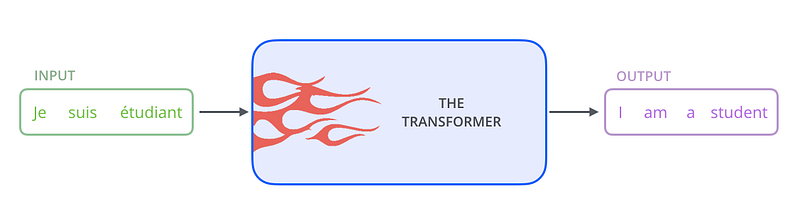
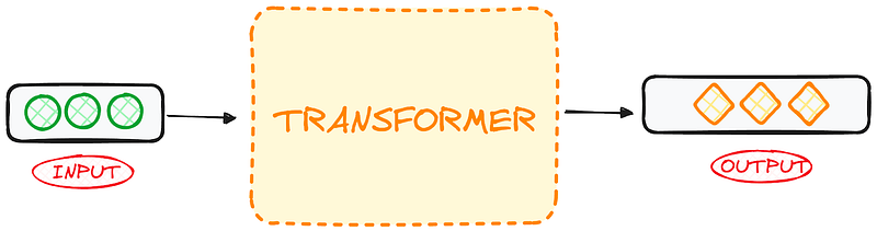
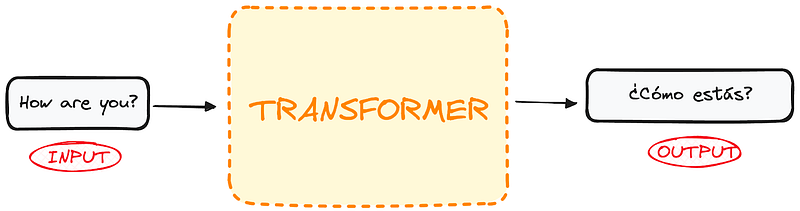
If we start considering a Transformer for language translation as a simple black box, it would take a sentence in one language, English for instance, as an input and output its translation in English.

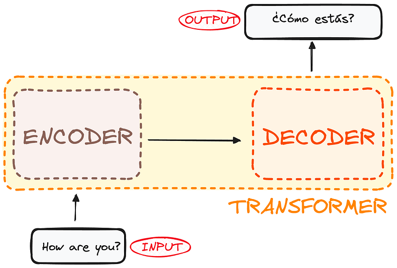
If we dive a little bit, we observe that this black box is composed of two main parts:

• The encoder takes in our input and outputs a matrix representation of that input. For instance, the English sentence “How are you?”
• The decoder takes in that encoded representation and iteratively generates an output. In our example, the translated sentence “¿Cómo estás?”

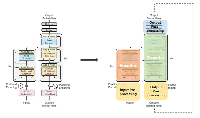
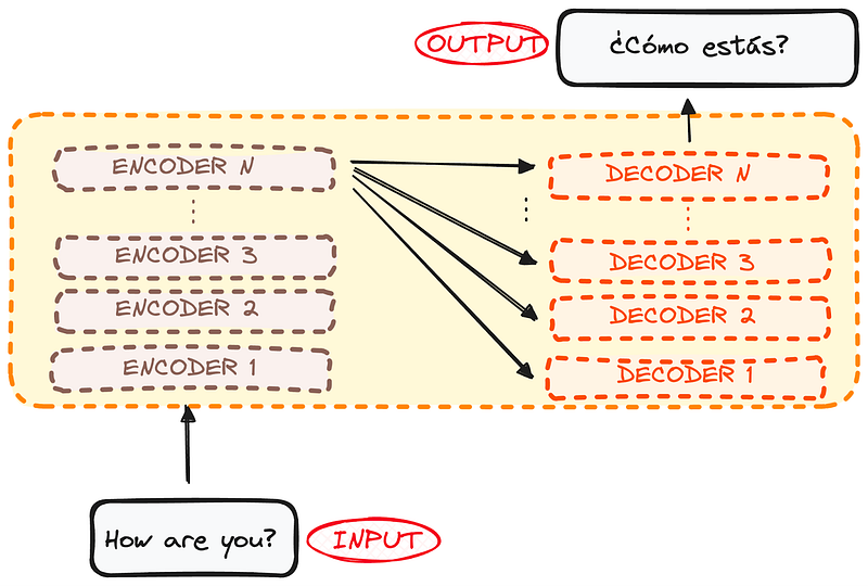
However, both the encoder and the decoder are actually a stack with multiple layers (same number for each). All encoders present the same structure, and the input gets into each of them and is passed to the next one. All decoders present the same structure as well and get the input from the last encoder and the previous decoder.

The original architecture consisted of 6 encoders and 6 decoders, but we can replicate as many layers as we want. So let’s assume N layers of each.

So now that we have a generic idea of the overall Transformer architecture, let’s focus on both Encoders and Decoders to understand better their working flow:

2.1 Embedding

The encoder is a fundamental component of the Transformer architecture. The primary function of the encoder is to transform the input tokens into contextualized representations. Unlike earlier models that processed tokens independently, the Transformer encoder captures the context of each token with respect to the entire sequence.

Its structure composition consists as follows:

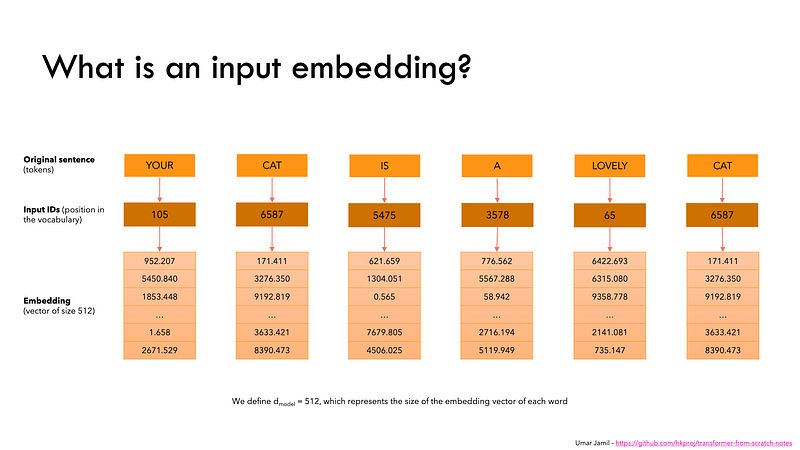
Text input is divided into smaller units called tokens, which can be words or subwords. These tokens are converted into numerical vectors called embeddings, which capture the semantic meaning of words.

2.1.1 Input Embedding

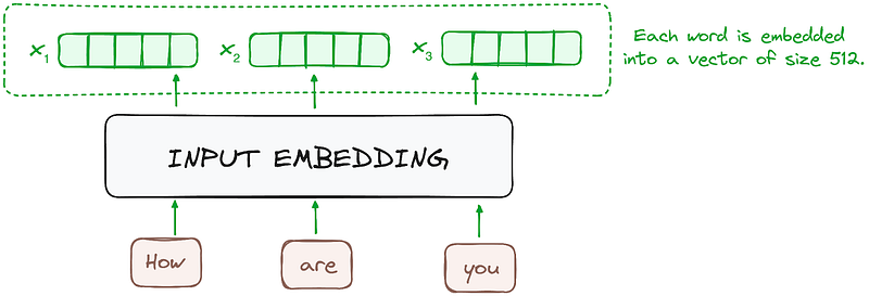
Let’s say you want to generate text using a Transformer model. You add the prompt like this one: “Data visualization empowers users to”. This input needs to be converted into a format that the model can understand and process. That is where embedding comes in: it transforms the text into a numerical representation that the model can work with. To convert a prompt into embedding, we need to

1. Tokenize the input,
2. Obtain token embeddings,
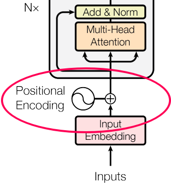
3. Add positional information, and finally
4. Add up token and position encodings to get the final embedding.

Let’s see how each of these steps is done.

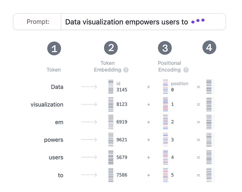
So let’s break its workflow into its most basic steps:

Step 1: Tokenization

Tokenization is the process of breaking down the input text into smaller, more manageable pieces called tokens. These tokens can be a word or a subword. The words "Data" and "visualization" correspond to unique tokens, while the word "empowers" is split into two tokens. The full vocabulary of tokens is decided before training the model: GPT-2's vocabulary has 50,257 unique tokens. Now that we split our input text into tokens with distinct IDs, we can obtain their vector representation from embeddings.

Step 2: Token Embedding

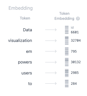
The embedding only happens in the bottom-most encoder. The encoder begins by converting input tokens — words or subwords — into vectors using embedding layers. These embeddings capture the semantic meaning of the tokens and convert them into numerical vectors.

All the encoders receive a list of vectors, each of size 512 (fixed-sized). In the bottom encoder, that would be the word embeddings, but in other encoders, it would be the output of the encoder that’s directly below them.

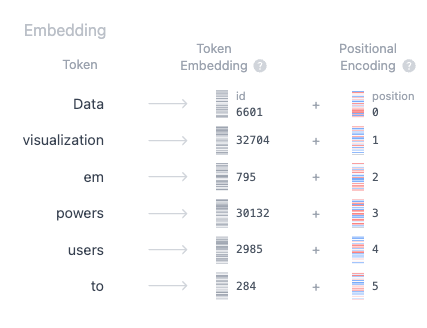
Step 3: Positional Encoding

The best part of the self-attention mechanism is its ability to generate dynamic contextual embeddings based on the context in which a particular word is used. Additionally, a major advantage of self-attention is that it allows all contextual embeddings to be calculated in parallel, making it possible to process large documents quickly. However, this parallel processing comes with a significant drawback: the self-attention module cannot capture the order of words in a sentence. For example, consider these two sentences:

1. Ravi killed the lion.
2. The lion killed Ravi.

If you pass both sentences through a self-attention block, it won’t be able to distinguish between them, as it doesn’t capture the order of the words.

This limitation can lead to misunderstandings in meaning, as the module treats sentences with the same words in different orders as identical. Positional encodings are introduced in the transformer architecture to address this issue. Positional encodings provide information about the order of words in a sentence, ensuring that the model understands the sequence and maintains the correct context.

The solution to positional encoding can be approached by addressing issues step-by-step. Initially, when processing a sentence like “Ravi killed the lion,” self-attention mechanisms do not inherently understand word order. A basic solution is assigning position numbers (e.g., “Ravi” = 1, “killed” = 2) and embedding these into word embeddings. However, this introduces several problems:

1. Unbounded Growth of Numbers: Large position numbers (e.g., 100,000 in a book) destabilize neural network training, leading to issues like vanishing or exploding gradients. Even normalizing these numbers causes inconsistencies across sentences of different lengths.

2. Discrete Numbers: Neural networks struggle with discrete numbers, as they prefer smooth, continuous values. Discrete values can cause numerical instability during training.

3. Inability to Capture Relative Positions: The approach only captures absolute positions but fails to understand relative distances between words, crucial for tasks in NLP.

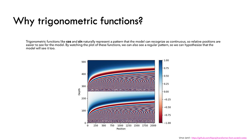
To address these, a solution requires a function that is bounded, continuous, and periodic, enabling the model to capture both absolute and relative positions effectively. This leads to the concept of positional encoding.

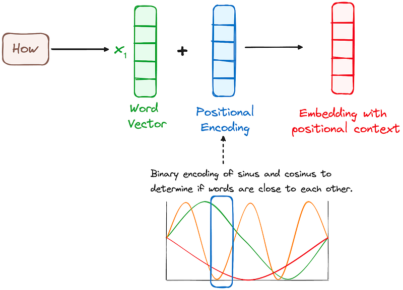
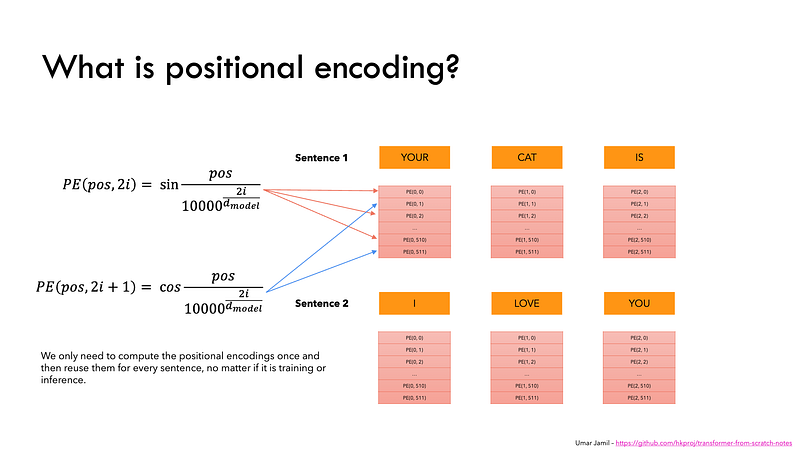
To do so, the researchers suggested employing a combination of various sine and cosine functions to create positional vectors, enabling the use of this positional encoder for sentences of any length.

In this approach, each dimension is represented by unique frequencies and offsets of the wave, with the values ranging from -1 to 1, effectively representing each position.

Step 4: Final Embedding

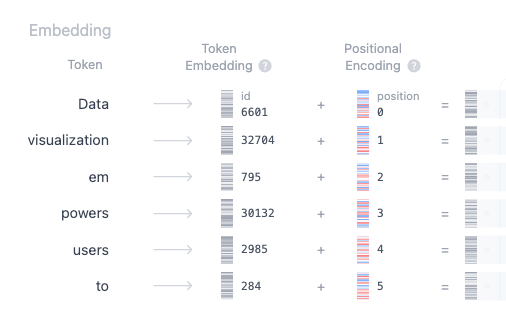
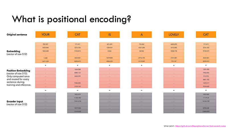
Finally, we sum the token and positional encodings to get the final embedding representation. This combined representation captures both the semantic meaning of the tokens and their position in the input sequence.

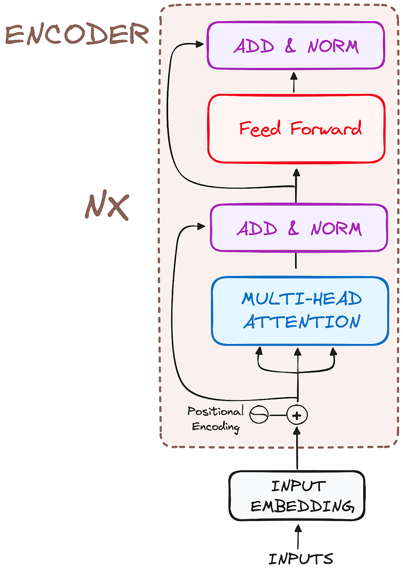
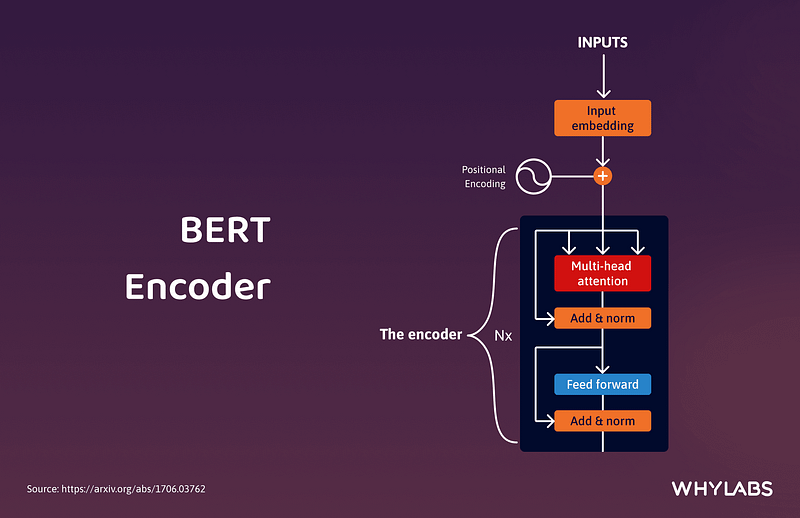
2.2 The Encoder

Stack of Encoder Layers

The Transformer encoder consists of a stack of identical layers (6 in the original Transformer model). This number was achieved through experimentation, giving the best results for various tasks.

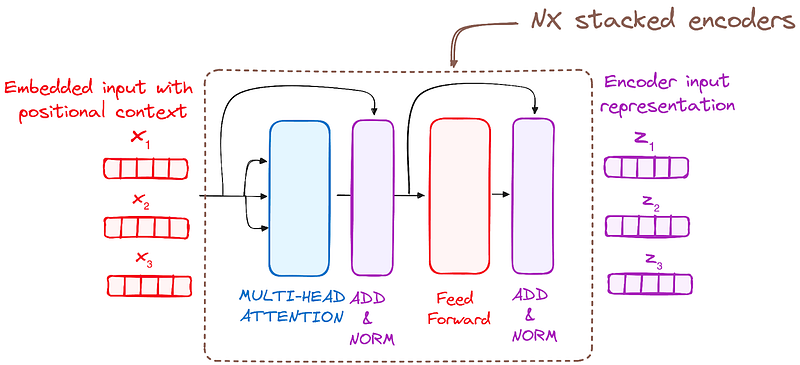
The encoder layer serves to transform all input sequences into a continuous, abstract representation that encapsulates the learned information from the entire sequence. This layer comprises two sub-modules:

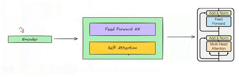
• A multi-headed attention mechanism.
• A fully connected network.

But how do these blocks work together? The actual architecture of an encoder block includes additional components like add & norm layers and residual connections. These ensure the flow of information remains smooth as it passes through each block.

The input data, typically a batch of sentences, enters the first encoder block, undergoes processing, and the output moves to the next encoder block. This process continues across all six encoder blocks, with the final output being passed to the decoder. Each block processes the data similarly, making the entire architecture highly efficient and structured.

In short, it incorporates residual connections around each sublayer, which are then followed by layer normalization.

2.2.1 Multi-Headed Self-Attention

The self-attention mechanism enables the model to focus on relevant parts of the input sequence, allowing it to capture complex relationships and dependencies within the data. Let’s look at how this self-attention is computed step-by-step.

Query, Key, and Value Matrices

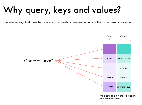
Each token’s embedding vector is transformed into three vectors: Query (Q), Key (K), and Value (V). These vectors are derived by multiplying the input embedding matrix with learned weight matrices for Q, K, and V. Here’s a web search analogy to help us build some intuition behind these matrices:

• Query (Q) is the search text you type in the search engine bar. This is the token you want to “find more information about”.
• Key (K) is the title of each web page in the search result window. It represents the possible tokens the query can attend to.
• Value (V) is the actual content of web pages shown. Once we matched the appropriate search term (Query) with the relevant results (Key), we want to get the content (Value) of the most relevant pages.

By using these QKV values, the model can calculate attention scores, which determine how much focus each token should receive when generating predictions.

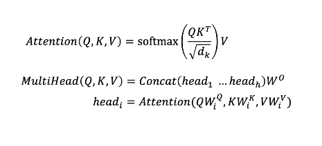
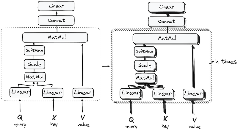
This first Self-Attention module enables the model to capture contextual information from the entire sequence. Instead of performing a single attention function, queries, keys and values are linearly projected h times. On each of these projected versions of queries, keys and values the attention mechanism is performed in parallel, yielding h-dimensional output values.

The detailed architecture goes as follows:

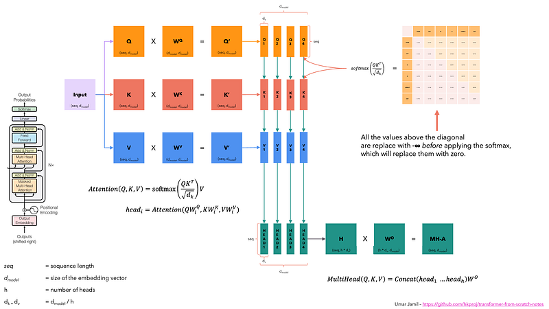
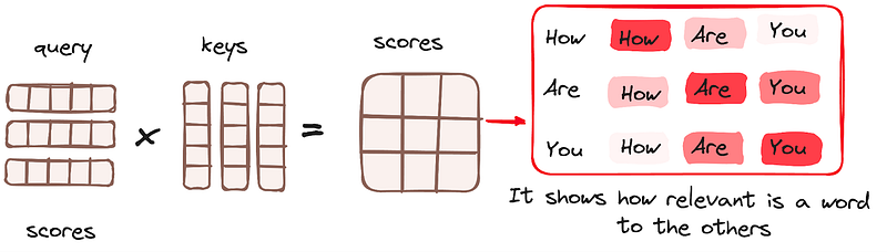
Once the query, key, and value vectors are passed through a linear layer, a dot product matrix multiplication is performed between the queries and keys, resulting in the creation of a score matrix.

The score matrix establishes the degree of emphasis each word should place on other words. Therefore, each word is assigned a score in relation to other words within the same time step. A higher score indicates greater focus.

This process effectively maps the queries to their corresponding keys.

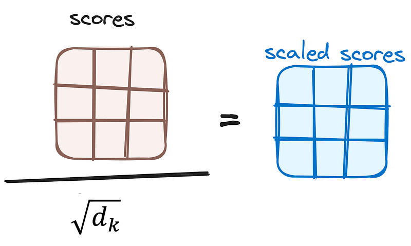
Reducing the Magnitude of attention scores

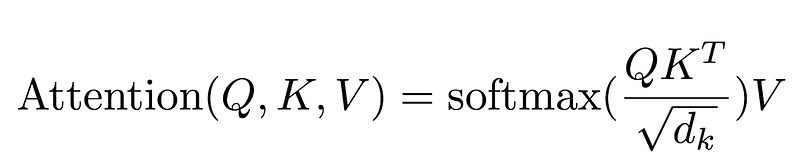
The scores are then scaled down by dividing them by the square root of the dimension of the query and key vectors. This step is implemented to ensure more stable gradients, as the multiplication of values can lead to excessively large effects.

Applying Softmax to the Adjusted Scores

Subsequently, a softmax function is applied to the adjusted scores to obtain the attention weights. This results in probability values ranging from 0 to 1. The softmax function emphasizes higher scores while diminishing lower scores, thereby enhancing the model’s ability to effectively determine which words should receive more attention.

Combining Softmax Results with the Value Vector

The following step of the attention mechanism is that weights derived from the softmax function are multiplied by the value vector, resulting in an output vector.

In this process, only the words that present high softmax scores are preserved. Finally, this output vector is fed into a linear layer for further processing.

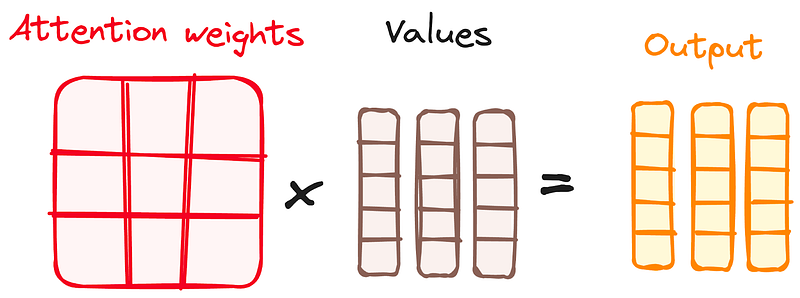
And we finally get the output of the Attention mechanism!

So, you might be wondering why it’s called Multi-Head Attention?

Remember that before all the process starts, we break our queries, keys and values h times. This process, known as self-attention, happens separately in each of these smaller stages or ‘heads’. Each head works its magic independently, conjuring up an output vector.

This ensemble passes through a final linear layer, much like a filter that fine-tunes their collective performance. The beauty here lies in the diversity of learning across each head, enriching the encoder model with a robust and multifaceted understanding.

2.2.2 Normalization and Residual Connections

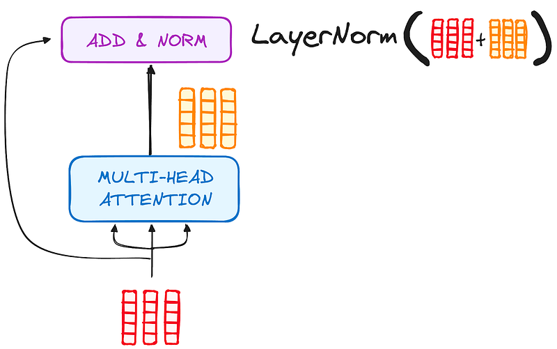
Each sub-layer in an encoder layer is followed by a normalization step. Also, each sub-layer output is added to its input (residual connection) to help mitigate the vanishing gradient problem, allowing deeper models. This process will be repeated after the Feed-Forward Neural Network too.

2.2.3 Feed-Forward Neural Network

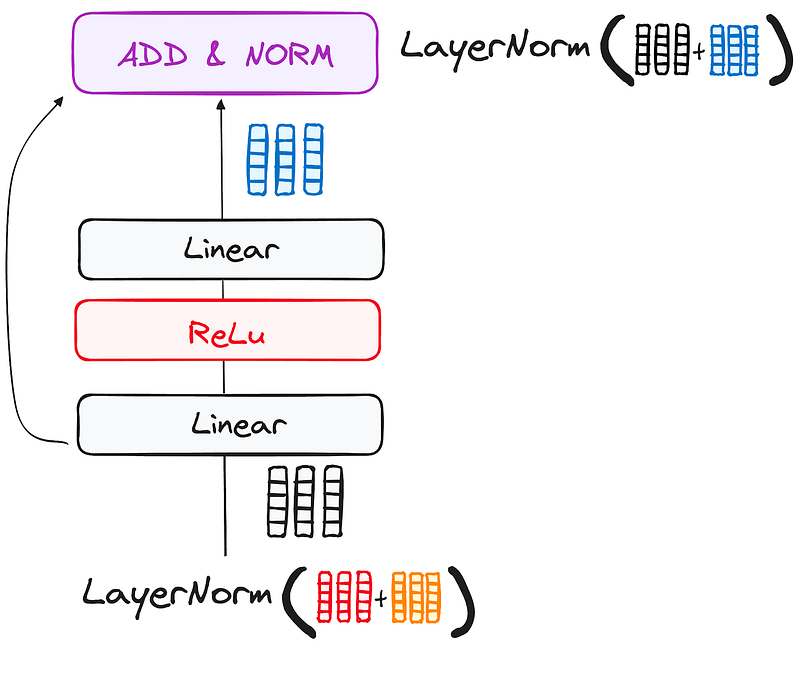
The journey of the normalized residual output continues as it navigates through a pointwise feed-forward network, a crucial phase for additional refinement.

Picture this network as a duo of linear layers, with a ReLU activation nestled in between them, acting as a bridge. Once processed, the output embarks on a familiar path: it loops back and merges with the input of the pointwise feed-forward network.

This reunion is followed by another round of normalization, ensuring everything is well-adjusted and in sync for the next steps.

2.2.4 Output of the Encoder

The output of the final encoder layer is a set of vectors, each representing the input sequence with a rich contextual understanding. This output is then used as the input for the decoder in a Transformer model.

This careful encoding paves the way for the decoder, guiding it to pay attention to the right words in the input when it’s time to decode.

Think of it like building a tower, where you can stack up N encoder layers. Each layer in this stack gets a chance to explore and learn different facets of attention, much like layers of knowledge. This not only diversifies the understanding but could significantly amplify the predictive capabilities of the transformer network.

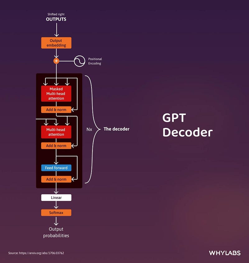
2.3 The Decoder

The decoder’s role centers on crafting text sequences. Mirroring the encoder, the decoder is equipped with a similar set of sub-layers. It boasts two multi-headed attention layers, a pointwise feed-forward layer, and incorporates both residual connections and layer normalization after each sub-layer.

These components function in a way akin to the encoder’s layers, yet with a twist: each multi-headed attention layer in the decoder has its unique mission.

The final of the decoder’s process involves a linear layer, serving as a classifier, topped off with a softmax function to calculate the probabilities of different words.

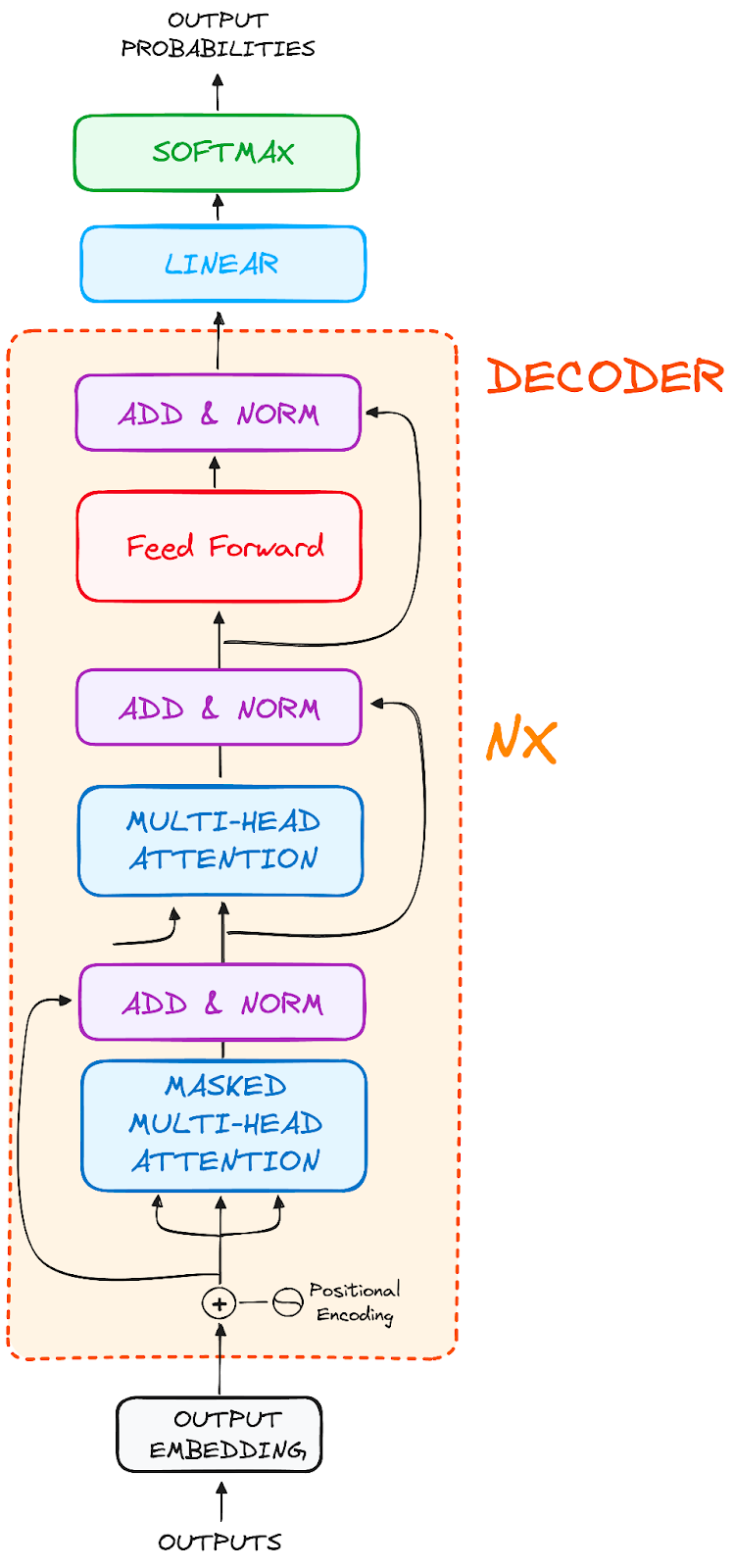
The Transformer decoder has a structure specifically designed to generate this output by decoding the encoded information step by step.

It is important to notice that the decoder operates in an autoregressive manner, kickstarting its process with a start token. It cleverly uses a list of previously generated outputs as its inputs, in tandem with the outputs from the encoder that are rich with attention information from the initial input.

This sequential dance of decoding continues until the decoder reaches a pivotal moment: the generation of a token that signals the end of its output creation.

2.3.1 Output Embeddings

At the decoder’s starting line, the process mirrors that of the encoder. Here, the input first passes through an embedding layer

2.3.2 Positional Encoding

Following the embedding, again just like the decoder, the input passes by the positional encoding layer. This sequence is designed to produce positional embeddings.

These positional embeddings are then channeled into the first multi-head attention layer of the decoder, where the attention scores specific to the decoder’s input are meticulously computed.

2.3.3 Stack of Decoder Layers

The decoder consists of a stack of identical layers (6 in the original Transformer model). Each layer has three main sub-components:

1. Masked Self-Attention Mechanism

This is similar to the self-attention mechanism in the encoder but with a crucial difference: it prevents positions from attending to subsequent positions, which means that each word in the sequence isn’t influenced by future tokens.

For instance, when the attention scores for the word “are” are being computed, it’s important that “are” doesn’t get a peek at “you”, which is a subsequent word in the sequence.

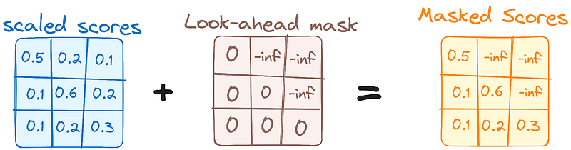
This masking ensures that the predictions for a particular position can only depend on known outputs at positions before it.

2. Encoder-Decoder Multi-Head Attention or Cross Attention

In the second multi-headed attention layer of the decoder, we see a unique interplay between the encoder and decoder’s components. Here, the outputs from the encoder take on the roles of both queries and keys, while the outputs from the first multi-headed attention layer of the decoder serve as values.

This setup effectively aligns the encoder’s input with the decoder’s, empowering the decoder to identify and emphasize the most relevant parts of the encoder’s input.

Following this, the output from this second layer of multi-headed attention is then refined through a pointwise feedforward layer, enhancing the processing further.

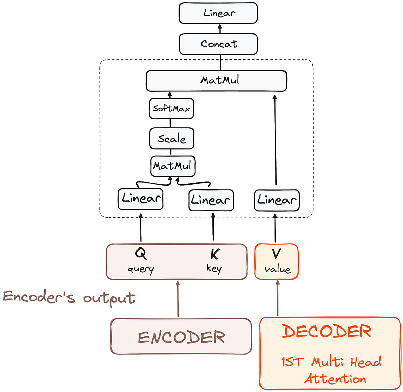
In this sub-layer, the queries come from the previous decoder layer, and the keys and values come from the output of the encoder. This allows every position in the decoder to attend over all positions in the input sequence, effectively integrating information from the encoder with the information in the decoder.

3. Feed-Forward Neural Network

Similar to the encoder, each decoder layer includes a fully connected feed-forward network, applied to each position separately and identically.

2.3.4 Linear Classifier and Softmax for Generating Output Probabilities

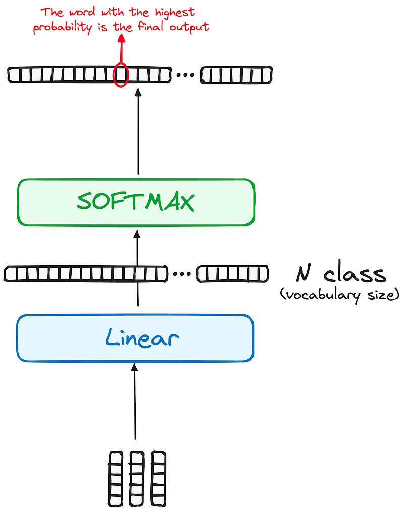
The journey of data through the transformer model culminates in its passage through a final linear layer, which functions as a classifier.

The size of this classifier corresponds to the total number of classes involved (number of words contained in the vocabulary). For instance, in a scenario with 1000 distinct classes representing 1000 different words, the classifier’s output will be an array with 1000 elements.

This output is then introduced to a softmax layer, which transforms it into a range of probability scores, each lying between 0 and 1. The highest of these probability scores is key,its corresponding index directly points to the word that the model predicts as the next in the sequence.

2.3.5 Normalization and Residual Connections

Each sub-layer (masked self-attention, encoder-decoder attention, feed-forward network) is followed by a normalization step, and each also includes a residual connection around it.

2.3.6 Output of the Decoder

The final layer’s output is transformed into a predicted sequence, typically through a linear layer followed by a softmax to generate probabilities over the vocabulary.

The decoder, in its operational flow, incorporates the freshly generated output into its growing list of inputs, and then proceeds with the decoding process. This cycle repeats until the model predicts a specific token, signaling completion.

The token predicted with the highest probability is assigned as the concluding class, often represented by the end token.

Again remember that the decoder isn’t limited to a single layer. It can be structured with N layers, each one building upon the input received from the encoder and its preceding layers. This layered architecture allows the model to diversify its focus and extract varying attention patterns across its attention heads.

Such a multi-layered approach can significantly enhance the model’s ability to predict, as it develops a more nuanced understanding of different attention combinations.

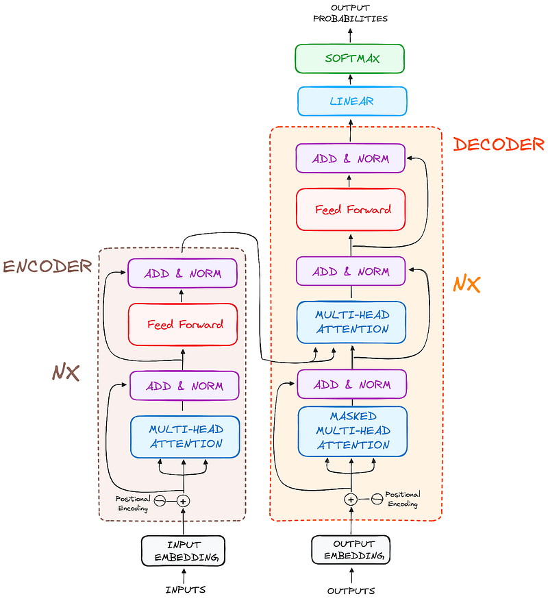
And the final architecture is something similar like this (form the original paper)

3. LLM Architectures

Architecture in machine learning (ML) refers to a model’s arrangement of neurons and layers. It’s like a blueprint that outlines how the model will learn from the data. Different architectures capture different relationships in the data that emphasize specific components during training. Consequently, the architecture influences the tasks the model is proficient in and the quality of the output it generates.

3.1 Seq-2-Seq Models (Encoder-decoder)

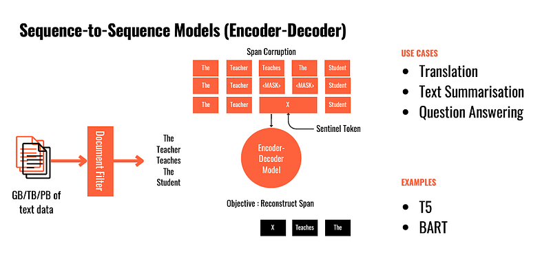
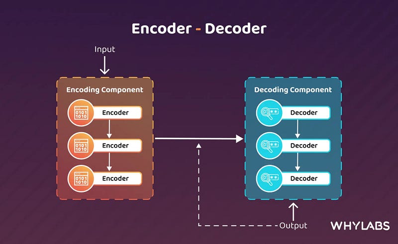
The Encoder-decoder consists of two components:

• Encoder — accepts the input data and converts it into an abstract continuous representation that captures the main characteristics of the input.
• Decoder — translates the continuous representation into intelligible outputs while ingesting its previous outputs.

The encoding and decoding process allows the model to handle complex language tasks through a more efficient representation of the data, which helps the model respond with coherence.

This dual-process architecture excels in generative tasks like machine translation (converting the same sentence from one language to another) and text summarization (summarizing the same key points in the text), where comprehending the entire input before generating output is crucial. However, it can be slower in inference due to the need to process the holistic input first.

LLM examples:

• Google’s — T5, Flan-UL2, and Flan-T5.
• Meta’s BART.

3.2 AutoEncoding Models (Encoder-only)

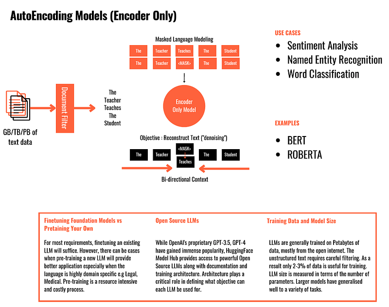
Models like the popular BERT (“Pre-training of Deep Bidirectional Transformers for Language Understanding,” 2018) and RoBERTa (“A Robustly Optimized BERT Pretraining Approach,” 2018) use encoder-only architectures to turn input into rich, contextualized representations without directly generating new sequences.

BERT, for instance, is pre-trained on extensive text corpora using two innovative approaches: masked language modeling (MLM) and next-sentence prediction. MLM works by hiding random tokens in a sentence and training the model to predict these tokens from their context. In this way, the model understands the relationship between words in both left and right contexts. This “bidirectional” understanding is crucial for tasks requiring strong language understanding, such as sentence classification (e.g., sentiment analysis) or fill missing words.

But unlike encoder-decoder models that can interpret and generate text, they don’t natively generate long text sequences. They focus more on interpreting input.

LLM examples:

• Google’s BERT and ALBERT.
• Meta’s RoBERTa.
• Microsoft’s DeBERTa.

3.3 AutoRegressive Models (Decoder-only)

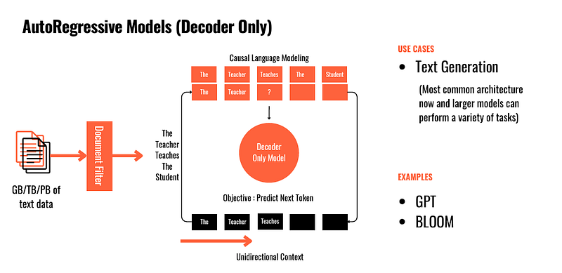
Decoder-only architectures generate the next part of the input sequence based on the previous context. Unlike encoder-based models, they cannot comprehend the entire input but excel at generating the next probable word. As such, Decoder-Only models are more “creative” and “open-ended” in their output.

This token-by-token output generation is effective for text-generation tasks like creative writing, dialogue generation, and story completion.

LLM examples:

• Open AI’s GPT-4 and GPT-3 series.
• Google’s PaLM and Bard.
• Meta’s LLaMA and OPT.

3.4 Mixture of Experts (MoE)

MoE, adopted by models like Mistral 8x7B, diverges from traditional Transformer models and builds upon the observation that a single monolithic language model can be decomposed into smaller, specialized sub-models. A gating network that distributes tasks (such as switching input tokens) among the models coordinates these sub-models, which concentrate on various aspects of the input data.

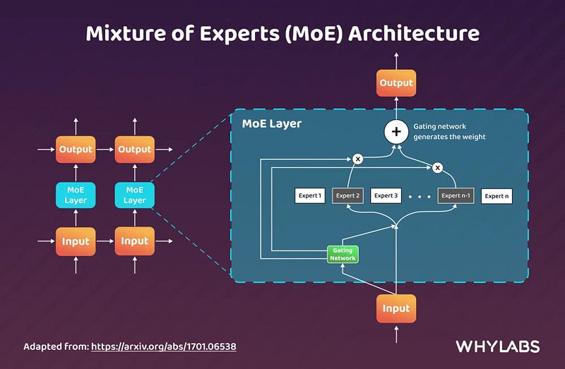
This approach enables scaling (efficient computation and resource allocation) and varied skills, which makes MoE great at handling complex tasks with varying requirements. The entire purpose of this architecture is to improve the number of LLM parameters without a corresponding increase in computational expense.

So, is Mistral 8x7B considered an LLM? Despite its architectural divergence from transformer models, it still qualifies as an LLM due to several reasons:

• Model size: Its enormous size and parameter count — 187 billion parameters — make it comparable to other LLMs in complexity and capacity.
• Pretraining: Like other LLMs, Mistral 8x7B is pre-trained on comprehensive datasets through unsupervised learning techniques, allowing it to understand and mimic human-like language patterns.
• Versatility: It demonstrates proficiency across various tasks, exhibiting LLMs’ broad range of capabilities.
• Adaptability: Like other LLMs, Mistral 8x7B can also be fine-tuned for specific tasks, enhancing performance.

4. Inference

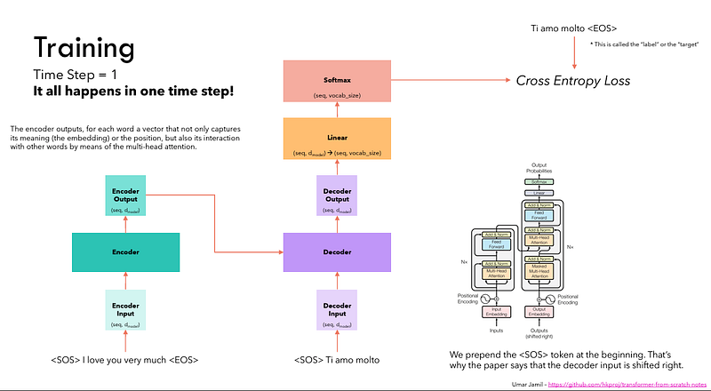
Now that we’ve covered the architecture of transformers and understood the components in detail, it’s time to discuss how inference is actually performed. We’ve trained our transformer model, and now, at the prediction phase, the architecture behaves slightly differently than it does during training.

Main difference between Training and Inference:

Training: Trains the Transformer model to learn patterns and relationships within the input data (e.g., language modeling, translation, etc.).

Inference: Uses the trained Transformer model to make predictions, such as generating text, translating languages, or classifying text.

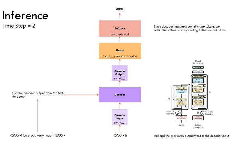
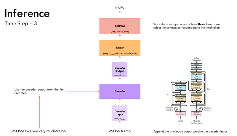
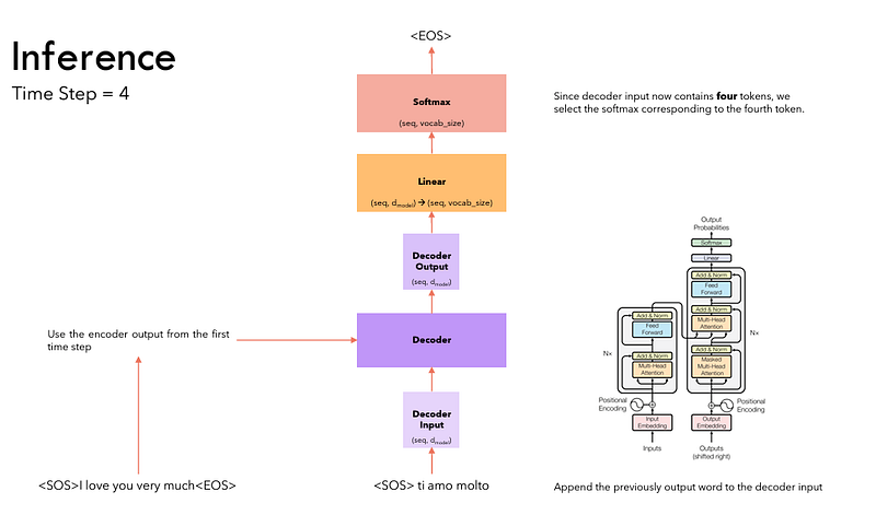
During inference, the main difference occurs in the decoder. Unlike training, where we already know the entire output sentence and can pass all tokens to the decoder at once, causing it to function in a non-autoregressive manner, during inference, we don’t have the full output sentence upfront. Therefore, the decoder must generate the translation one word at a time in an autoregressive fashion. It uses each previously predicted word to help predict the next word in the sequence. This process continues until the model generates the entire translated sentence.

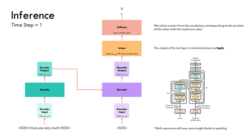
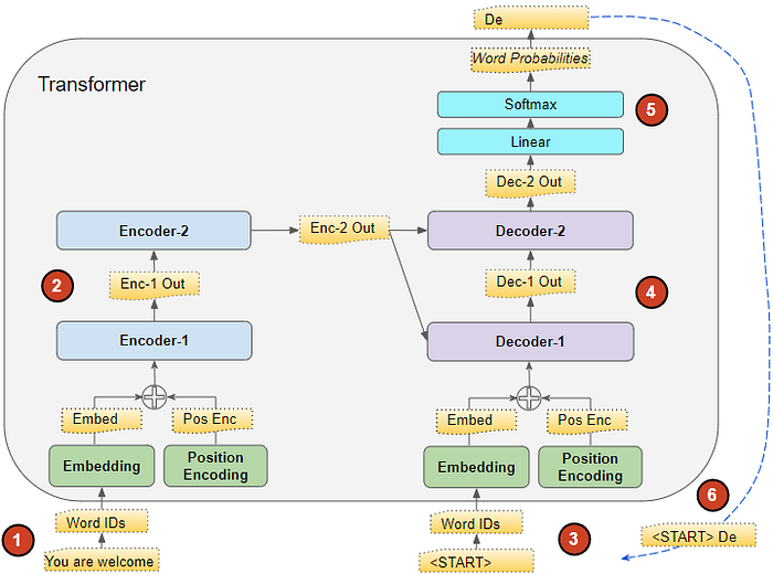
The flow of data during Inference is:

1. The input sequence is converted into Embeddings (with Position Encoding) and fed to the Encoder.
2. The stack of Encoders processes this and produces an encoded representation of the input sequence.
3. Instead of the target sequence, we use an empty sequence with only a start-of-sentence token. This is converted into Embeddings (with Position Encoding) and fed to the Decoder.
4. The stack of Decoders processes this along with the Encoder stack’s encoded representation to produce an encoded representation of the target sequence.
5. The Output layer converts it into word probabilities and produces an output sequence.
6. We take the last word of the output sequence as the predicted word. That word is now filled into the second position of our Decoder input sequence, which now contains a start-of-sentence token and the first word.
7. Go back to step #3. As before, feed the new Decoder sequence into the model. Then take the second word of the output and append it to the Decoder sequence. Repeat this until it predicts an end-of-sentence token. Note that since the Encoder sequence does not change for each iteration, we do not have to repeat steps #1 and #2 each time

4.1 Inference Techniques

The Transformer can be used for inference by feeding it a sequence of tokens one at a time. The encoder is used to process the input sequence and produce a sequence of embeddings. The decoder is used to generate the output sequence one token at a time. The decoder uses the encoder output and the previously generated tokens to generate the next token. The Transformer can use different strategies for inference, such as greedy search and beam search.

4.1.1 Greedy Search

Greedy search is a simple strategy for inference. At each time step, the decoder generates the token that has the highest probability according to its model. This process is repeated until the decoder generates an end-of-sequence token. Greedy search is fast but can get stuck in local optima.

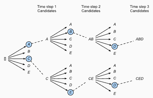
4.1.2 Beam Search

Beam search is a more sophisticated strategy for inference. At each time step, the decoder generates a beam of tokens, where the beam size is a hyperparameter. The decoder then selects the top-k tokens from the beam and continues to generate tokens from each of these tokens. This process is repeated until the decoder generates an end-of-sequence token. Beam search is slower than greedy search but can generate more diverse and accurate outputs.

There are other strategies for inference that can be used with the Transformer, such as sampling and nucleus sampling. These strategies can be used to generate more creative and diverse outputs.

5. Transformer Inference Optimization

Transformer models, known for their self-attention mechanisms, are central to tasks like NLP and computer vision. Inference, the phase where these models generate predictions on unseen data, requires significant computational resources.

One key factor affecting transformer inference is the number of floating-point operations (FLOPs). Each layer involves matrix multiplications, and for large models like GPT-3, this can amount to trillions of FLOPs per token. To reduce computational overhead, Key-Value (KV) caching is used, allowing the model to reuse previously computed attention vectors, speeding up autoregressive decoding.

Memory usage is another constraint, with models like GPT-3 demanding over 200 GB of memory. Techniques like quantization and parallelism help manage these resources more efficiently, but transformer inference often remains memory-bound, where memory bandwidth limits the speed of computation.

5.1 Transformer Architecture and Inference Flow

The core architecture of transformers is based on the self-attention mechanism and a series of stacked layers, each comprising attention and feed-forward networks. During inference, transformers apply pre-trained parameters to make predictions, typically token by token in autoregressive models like GPT.

Inference involves several matrix operations, particularly matrix-vector multiplications in each attention layer. For each new token, the model computes query (Q), key (K), and value (V) vectors by multiplying input embeddings with learned weight matrices.

The attention mechanism calculates relevance scores by multiplying the query with the transposed key matrix, scaling the result by the square root of the dimension size, and applying a softmax function. This process allows the model to weigh the importance of each token in the sequence. While highly effective, these matrix multiplications are computationally expensive, particularly in large models like GPT-3 or LLaMA, where each attention head performs billions of FLOPs per token.

5.2 Phases of Transformer Inference: Prefill and Decode

Transformer inference operates in two key phases: prefill and decode. These phases dictate how the model processes input tokens and generates output tokens, with different performance implications for each.

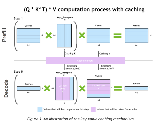
1. Prefill Phase: In the prefill phase, the model processes the entire input sequence in parallel, transforming tokens into key-value pairs. This phase is computationally intensive but highly parallelizable, enabling efficient GPU utilization. Operations primarily involve matrix-matrix multiplications, allowing the GPU to handle multiple tokens simultaneously. Prefill excels in batch processing, where large amounts of data can be processed together, minimizing latency.

2. Decode Phase: The decode phase is more memory-bound and sequential, generating tokens one by one. Each new token depends on the previously generated tokens, requiring matrix-vector multiplications, which underutilizes the GPU compared to the parallel nature of the prefill phase. The sequential process introduces latency bottlenecks, making this phase significantly slower, especially in large models like GPT-3.

Key-Value (KV) Caching is a critical optimization in the decode phase. By storing previously computed key-value matrices, the model avoids recomputation, reducing complexity from quadratic to linear.

6. Challenges in Transformer Inference

Large transformer models, especially Large Language Models (LLMs) like GPT-3, introduce several challenges during inference due to their size and compute requirements. These challenges revolve around memory limitations, latency, and balancing between memory-bound and compute-bound operations.

1. Memory and Computational Demands: Storing both model weights and the key-value (KV) cache during inference requires vast amounts of memory. Large models like GPT-3, with 175 billion parameters, often need over 200 GB of memory. Additionally, the KV cache size grows linearly with sequence length and batch size, further increasing the memory burden. For instance, a LLaMA model with 7 billion parameters and a sequence length of 4096 can consume around 2 GB of memory just for the KV cache.

2. Latency in Sequential Token Generation: Latency is a critical issue, especially in the decode phase, where tokens are generated one at a time. Each new token depends on the previous one, which results in sequential operations that underutilize the GPU’s compute power. Even highly optimized models suffer from memory bandwidth bottlenecks, which become more pronounced as the sequence length increases.

3. Balancing Batch Size and Performance: Larger batch sizes can improve GPU utilization, especially during the prefill phase, but they are limited by memory capacity. Increasing batch size helps maximize throughput, but only up to the point where the system becomes memory-bound. Beyond this, the system may encounter diminishing returns, as memory bandwidth starts to limit further performance gains.

4. Trade-offs in Memory-Bound vs. Compute-Bound Operations: Transformer inference alternates between memory-bound and compute-bound operations. During the decode phase, matrix-vector multiplications are often memory-bound, while prefill matrix-matrix operations tend to be compute-bound. Effective optimization of batch size, KV cache management, and precision (e.g., FP16, INT8) is crucial for reducing latency and ensuring efficient GPU use.

7. Optimization Techniques for Faster Inference

As transformer models like GPT-3, LLaMA, and other large language models (LLMs) continue to scale, optimisation techniques have become essential for managing the increased memory, computational load, and latency associated with inference. By applying techniques like quantization, key-value (KV) caching, speculative decoding, batching, and parallelism, developers can significantly improve inference performance.

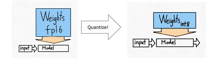
7.1 Quantization

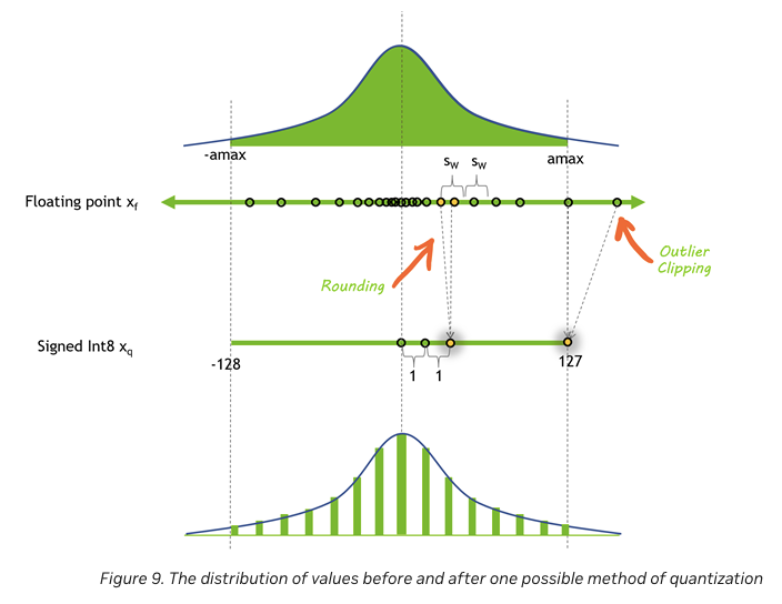
The distribution of values before and after quantization, illustrating the process of rounding and outlier clipping during the conversion from floating-point to INT8.Source:

Quantization reduces the precision of model weights and activations, allowing for faster computation and lower memory usage. Instead of relying on 32-bit or 16-bit floating-point precision, models can use 8-bit (INT8) or even lower, which reduces memory bandwidth and allows the model to handle larger batch sizes or longer sequences more efficiently.

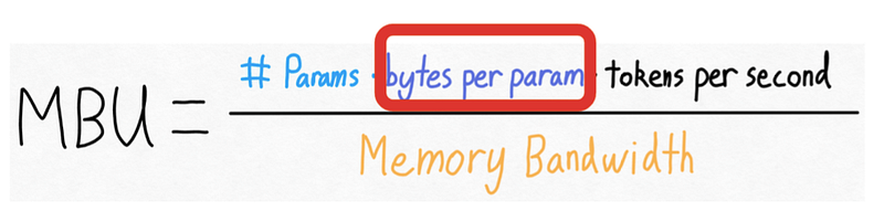
The Memory Bandwidth Utilization (MBU) formula shows how memory bandwidth limits performance, with the number of parameters, bytes per parameter, and tokens per second impacting inference speed

For example, applying INT8 quantization to GPT-3 can result in up to a 50% reduction in memory requirements, directly leading to lower latency and higher throughput during inference. Quantization is particularly useful for memory-bound models that face bandwidth limitations.

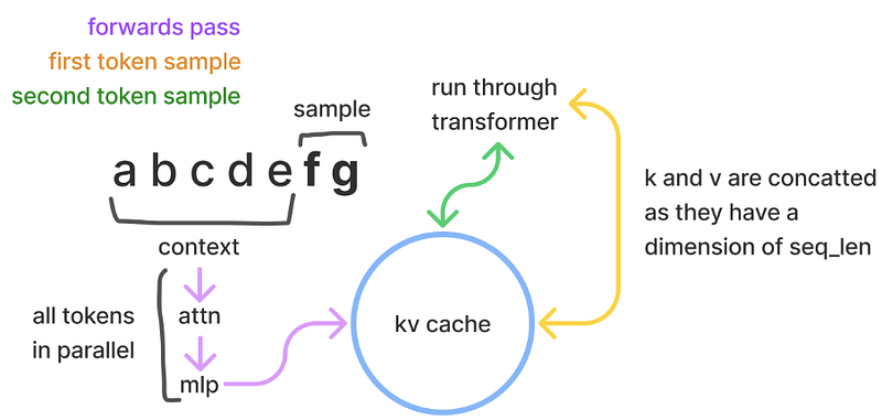
7.2 Key-Value (KV) Caching

In autoregressive models, each new token generation requires accessing all previous tokens. This leads to a quadratic increase in computations as the sequence length grows. KV caching mitigates this by storing key and value tensors from previous tokens, allowing the model to reuse them without recomputation.

The size of the KV cache grows linearly with the number of tokens, layers, and attention heads. For instance, in the LLaMA 7B model, a sequence length of 4096 tokens would require approximately 2 GB of memory for the KV cache. This optimization significantly reduces the computational load in the decode phase, improving both speed and memory efficiency.

7.3 Speculative Decoding

Speculative decoding is an advanced optimization technique that reduces latency by parallelizing token generation. Instead of waiting for each token to be processed sequentially, speculative decoding uses a smaller draft model to predict several tokens ahead, verifying the predictions with the main model. If the predictions are accurate, they are accepted; if not, they are discarded.

This approach allows for parallel execution, reducing the overall time required for token generation while maintaining accuracy. It’s especially useful for real-time applications, such as chatbots, where fast response times are crucial.

7.4 Batching

Batching is a straightforward yet powerful technique for optimizing transformer inference. By processing multiple inputs simultaneously, batching improves GPU utilization, as the memory cost of the model’s weights is shared across multiple requests. However, batching is limited by available memory, particularly in models with long sequences.

A challenge with traditional batching is that different requests within a batch may generate varying numbers of output tokens. This can lead to inefficiencies, as all requests must wait for the longest-running one to complete. To address this, in-flight batching allows the system to evict completed requests from the batch immediately, freeing up resources for new requests.

7.5 Hardware Optimisation: Parallelism

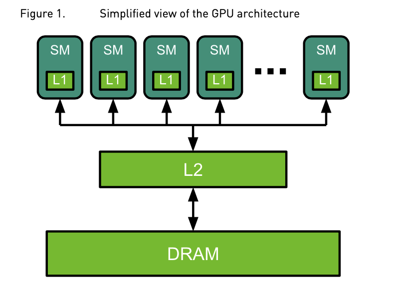
Hardware optimizations, particularly tensor parallelism and pipeline parallelism, are critical for scaling large models. These methods distribute the computational load across multiple GPUs, allowing systems to handle models that exceed the memory capacity of a single GPU.

· Tensor Parallelism: This technique splits a model’s parameters across multiple GPUs, enabling them to process different parts of the same input in parallel. Tensor parallelism is particularly effective for attention layers, where different attention heads can be computed independently.

· Pipeline Parallelism: This approach divides the model into sequential chunks, each processed by a different GPU. Pipeline parallelism reduces the memory footprint per GPU, allowing larger models to run efficiently. However, it introduces some idle time between GPUs while waiting for data from previous stages.

Both forms of parallelism are essential for managing large models like GPT-3 and LLaMA, where memory and computational demands often exceed the capabilities of a single GPU.

7.6 FlashAttention and Memory Efficiency

Another critical advancement is FlashAttention, which optimizes memory access patterns by reducing the number of times data is loaded and stored in memory. FlashAttention leverages GPU memory hierarchies to perform computations more efficiently, fusing operations and minimizing data movement. This technique can lead to significant speedups, especially in models with large sequence lengths, by reducing memory waste and enabling larger batch sizes.

8. Benchmarking Inference Performance

Benchmark tests for both GPT-3 and LLaMA illustrate the impact of these optimizations. For GPT-3, the combination of KV caching and quantization has been shown to reduce inference time by up to 60% compared to unoptimized models, with throughput reaching hundreds of tokens per second. In LLaMA, the use of parallelism techniques ensures that even the largest models, like LLaMA 65B, can maintain high throughput while keeping latency under control.

These optimizations allow both models to scale effectively, ensuring that they can handle real-world applications, from long-context generation to real-time responses, with significantly reduced computational and memory demands.

8.1 Trends in Transformer Inference

As transformer models continue to grow in size and complexity, optimizing inference is crucial for keeping up with the demands of real-world applications. The next wave of innovations focuses on scaling transformer models efficiently, improving memory management, and leveraging advanced hardware capabilities. Below are some of the most impactful trends shaping the future of transformer inference.

8.1.1 Memory Optimization with Paging and FlashAttention

A key trend is optimizing memory usage through techniques like PagedAttention and FlashAttention. In current inference processes, models often over-provision memory to handle the maximum possible sequence length, which leads to inefficiencies. PagedAttention addresses this by allocating memory only as needed, breaking the key-value (KV) cache into smaller blocks that are fetched on demand.

FlashAttention further enhances memory efficiency by optimizing the order of computations and reducing data movement between memory and compute units. By fusing operations and leveraging GPU memory hierarchies, FlashAttention can significantly reduce memory waste and enable larger batch sizes and faster processing. These advancements will be key to scaling large models while maintaining high performance.

8.1.2 Multi-Query and Grouped-Query Attention

Optimizing the attention mechanism itself is another important trend. Multi-Query Attention (MQA) and Grouped-Query Attention (GQA) are two variations that reduce the memory footprint while maintaining model performance. In MQA, all heads share the same key-value pairs, which reduces the size of the KV cache while preserving accuracy.

Grouped-Query Attention (GQA), which strikes a balance between MQA and traditional multi-head attention, uses shared key-value pairs for grouped heads. This approach further reduces memory usage while maintaining high performance, making it particularly useful for long-context models like LLaMA 2 70B.

8.1.3 Parallelism: Tensor and Sequence

Parallelism remains a central strategy for scaling large models. Tensor parallelism divides model layers into independent blocks that can be processed across multiple GPUs, reducing the memory burden on individual devices. This method works well for attention heads and feed-forward layers, where parallel processing can significantly boost efficiency.

vSequence parallelism further improves memory efficiency by splitting operations like LayerNorm and Dropout across the sequence dimension. This reduces memory overhead, particularly for long-sequence tasks, and allows models to scale more effectively.

8.1.4. Speculative Inference for Real-Time Applications

For real-time applications, speculative inference offers an innovative approach to reduce latency. By using smaller draft models to predict multiple tokens ahead, speculative inference allows for parallel execution. The draft tokens are then verified by the main model, which either accepts or discards them.

9. Handling Large Datasets

Training Transformers on large datasets poses unique challenges and requires careful strategies:

9.1 Efficient Data Loading and Preprocessing

• Parallel Data Loading: Utilizing frameworks like TensorFlow’s tf.data or PyTorch’s DataLoader with multi-threading speeds up data preprocessing.
• Shuffling and Batching: Proper shuffling prevents overfitting to any specific data order, and batching ensures efficient GPU utilization.

9.2 Distributed Training

• Data Parallelism: The model is replicated across multiple GPUs, each processing a different mini-batch of data, and gradients are aggregated.
• Model Parallelism: The model itself is split across multiple GPUs, useful for very large models that don’t fit into the memory of a single device.

9.3 Mixed Precision Training

• Leveraging 16-bit (half-precision) floating point operations instead of 32-bit significantly reduces memory usage and speeds up computation without a major impact on accuracy.

9.4 Gradient Accumulation

• Useful for scenarios where batch sizes are limited by GPU memory. Gradients are accumulated over multiple smaller batches before performing an optimizer step.

9.5 Checkpointing and Resuming

• Saving model states periodically during training helps resume from the last checkpoint in case of failures, and can also be used for early stopping and fine-tuning purposes.

9.6 Data Augmentation and Sampling

• Data augmentation techniques increase data variability, helping generalization.
• Smart sampling strategies ensure the model doesn’t overfit on common patterns while ignoring rare but important ones.

10. Conclusion

This blog delves into the development and optimization of Large Language Models (LLMs), beginning with an overview of their construction and training methods. It traces the evolution from pre-Transformer models to the transformative introduction of Transformers, emphasizing the pivotal “Attention is All You Need” concept.

The core of the blog dissects the Transformer architecture, detailing its components like embedding layers, encoder-decoder interactions, and self-attention mechanisms. It explores various LLM architectures, including Seq-2-Seq, AutoEncoding, and AutoRegressive models, shedding light on their distinct functionalities.

For practical deployment, the blog examines inference strategies, optimization techniques such as quantization, KV caching, speculative decoding, and hardware parallelism, with real-world examples like GPT-3 and LLaMA. Performance benchmarks, memory optimization, and parallelism techniques highlight trends in efficient Transformer inference.

Lastly, the blog addresses handling large datasets, discussing efficient data processing, distributed training, mixed precision techniques, and data augmentation strategies. This comprehensive guide serves as a deep dive into building, optimizing, and deploying LLMs effectively.

11. Test your Knowledge!

1. How do Transformers overcome the limitations of RNNs in handling long sequences?

Answer: Transformers use self-attention, enabling each token to interact with every other token in the sequence, capturing long-range dependencies more efficiently than RNNs, which suffer from vanishing/exploding gradients and slow processing for long sequences.

2. Explain the role of multi-head attention in the Transformer encoder.

Answer: Multi-head attention allows the model to focus on different parts of the input sequence simultaneously, enhancing its ability to capture diverse contextual relationships and features within the data.

3. What are key-value (KV) caches, and how do they optimize Transformer inference?

Answer: KV caches store computed key and value matrices during inference, allowing efficient reuse of attention scores across tokens, reducing redundant computations and speeding up decoding.

4. What is the significance of positional encoding in the Transformer model?

Answer: Since Transformers lack inherent sequence order awareness, positional encoding introduces token position information through sinusoidal functions, allowing the model to capture word order within sequences.

5. Describe how quantization is used to optimize Transformer inference.

Answer: Quantization reduces model precision, typically converting weights from 32-bit floating-point to lower-precision formats like 8-bit integers, reducing memory usage and computational cost while maintaining accuracy.

6. How do encoder-only (AutoEncoding) models differ from decoder-only (AutoRegressive) models in LLM architectures?

Answer: Encoder-only models excel at tasks requiring input sequence understanding (e.g., classification), while decoder-only models generate output token by token, making them effective for language generation tasks.

7. What is speculative decoding, and why is it used in Transformer inference?

Answer: Speculative decoding generates multiple tokens simultaneously during inference, then validates and adjusts them against the model’s predictions, reducing latency and speeding up real-time applications.

8. Explain the difference between greedy search and beam search for Transformer inference.

Answer: Greedy search selects the highest-probability token at each step, while beam search maintains multiple hypotheses, exploring a set number of likely sequences to find the best one based on cumulative probability.

9. How do residual connections and normalization layers benefit the Transformer architecture?

Answer: Residual connections help stabilize training by allowing gradients to flow through layers more effectively, while normalization layers improve convergence and ensure consistent input scaling for subsequent layers.

10. What techniques are employed to handle large datasets efficiently during LLM training?

Answer: Techniques include distributed training, efficient data loading, mixed precision training to reduce memory usage, gradient accumulation to manage large batch sizes, and checkpointing for fault tolerance and resumption.

11.1 DIY

1. What is the main difference between GPT and BERT series?
2. Explain the architecture of a transformer, what is your understanding about it?
3. How do you evaluate the performance of a transformer?
4. What is key-value pair in a transformer?
5. In a transformer, how are the probabilities obtained from the softmax function used to decide distribution or randomness?
6. Explain Multi GPU Training & Multi-Node Distributed Systems.
7. What is cross-attention?
8. What is the difference between layer and batch normalization?
9. How does Batch Norm & Layer behave during Train / Inference ?
10. Why do Encoders have Self-Attention and Decoders have Masked Self-Attention ?
11. Explain masking in transformers during training or inference?
12. Do transformers output probabilities depend only on previous tokens?
13. What is the masked multi-head attention layer responsible for?
14. Explain the difference between Quantization, Pruning & Distillation.

Credits

This blog post has compiled information from various sources, including research papers, technical blogs, official documentation, YouTube videos, and more. Each source has been appropriately credited beneath the corresponding images, with source links provided.

Below is a consolidated list of references:

1. https://towardsdatascience.com/transformers-141e32e69591
2. https://www.kaggle.com/code/lusfernandotorres/transformer-from-scratch-with-pytorch/code
3. https://deeprevision.github.io/posts/001-transformer/
4. https://poloclub.github.io/transformer-explainer/
5. https://nlp.seas.harvard.edu/annotated-transformer/
6. https://towardsdatascience.com/transformers-explained-visually-part-1-overview-of-functionality-95a6dd460452

Thank you for reading!

If this guide has enhanced your understanding of Python and Machine Learning:

• Please show your support with a clap 👏 or several claps!
• Your claps help me create more valuable content for our vibrant Python or ML community.
• Feel free to share this guide with fellow Python or AI / ML enthusiasts.
• Your feedback is invaluable — it inspires and guides my future posts.

Connect with me!

Vipra