Summary

The web content provides a tutorial on applying simple linear regression to time series data, specifically focusing on modeling mean temperature in Delhi, India, using time-step and lag features.

Abstract

The article is an installment in a data series, specifically episode 17.2, which guides readers through the process of implementing simple linear regression in the context of time series analysis. It emphasizes the engineering of two key features: a time-step feature that indexes dates with a numerical value to model time dependence, and a lag feature that shifts observations to predict based on past values, modeling serial dependence. The tutorial includes practical Python code using libraries such as pandas, NumPy, and scikit-learn to demonstrate data exploration, model training, and visualization of results. The author illustrates the use of these features with the example of predicting mean temperature in Delhi, India, over a four-year period, and concludes that a combination of time-step and lag features can improve time series models.

Opinions

The author suggests that reviewing previous episodes on linear regression is beneficial before proceeding with the current tutorial.
The article implies that simple linear regression might not always capture complex time dependencies, hinting at the potential need for more sophisticated time series models.
The author indicates that the inclusion of lag features is useful when there is a correlation between current and previous observations, which can enhance the predictive power of time series models.
The article encourages readers to engage by asking questions, fostering an interactive learning environment.
The recommendation of an AI service at the end of the article suggests the author's endorsement of cost-effective alternatives to premium AI platforms like ChatGPT Plus (GPT-4).

Simple Linear Regression with Time Series

Step-by-step follow-along | Data Series | Episode 17.2

Consider reviewing episodes on linear regression before continuing:

Overview

There are two features we can engineer for simple linear regression for time series analysis.

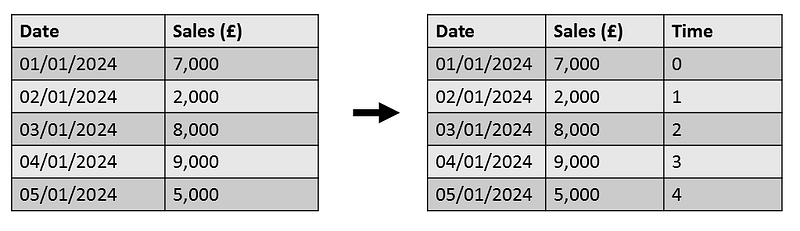
Time-step (Date Time) feature

We index each date with a time, for example:

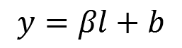
This enables us to produce the model:

Where:

y : is our target (sales)
β: is our weight
t: is our time-step feature
b: is our bias

Time-step features enable us to model time dependence. A time series is said to be time dependent if observations can be predicted based on the time in which it occurred.

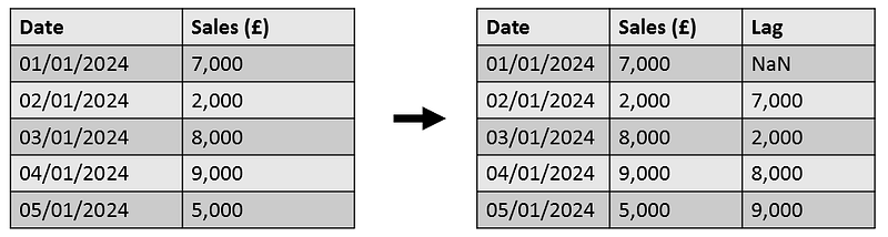
2. Lag feature

Another feature we can make for time series analysis, is something called the lag feature.

For this we shift all our observations so they occur later in time.

For example:

This enables us to produce a similar model as before, but for this case using lag as our feature instead of time.

Lag features enable us to model serial dependence. A time series is said to have serial dependence when an observation can be predicted from past observations.

— — — — —

In this episode we focus on applying simple linear regression to time series data to model the mean temperature in Delhi, India from 1st January 2013 to 1st January 2017.

Libraries

import pandas as pd
import warnings
import numpy as np
import matplotlib.pyplot as plt

warnings.filterwarnings("ignore")

Data Exploration

We read our data into python using the read_csv function from pandas.

# read the data
df = pd.read_csv("D:\ProjectData\weather_ts.csv")

# check data frame shape
df.shape

We can make use of the head function to view the first few rows of our dataframe:

df.head()

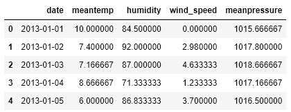
We have four variables that are being recorded against time:

1) Mean Temperature 2) Humidity 3) Wind Speed 4) Mean Pressure

For this episode we are going to be focussing on mean temperature.

Adding Time-step Feature

df['Time'] = np.arange(len(df.index))

df.head()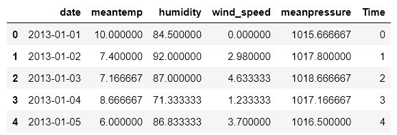

From the above output we observe each date has been indexed with a time.

from sklearn.linear_model import LinearRegression

# Training data
X_ts = df[["Time"]]  # feature
y_ts = df.meantemp  # target

# Train the model
model_ts = LinearRegression()
model_ts.fit(X_ts, y_ts)

# Generate a series of predicted values
y_pred_ts = pd.Series(model_ts.predict(X_ts))

To obtain our model intercept and coefficient we can use the following code:

model_ts.intercept_, model_ts.coef_

Which gives the model to 3dp:

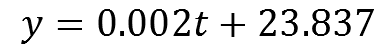
We can produce a plot of our time series data using the time step feature and add our regression line:

plt.figure(figsize=(11, 4))

# Plot the data points
plt.plot(X, y, marker='o', markersize=2, linestyle='-', label='Actual data')

# Plot the regression line
plt.plot(X, y_pred, color='red', label='Regression line')

# Add labels and a legend
plt.xlabel('Time')
plt.ylabel('Mean Temperature')
plt.title('Simple Linear Regression (Time-step)')
plt.legend()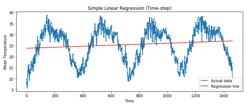

The above regression line does not capture the time dependence shown in our plot, a more complex time series model might be needed.

Lag feature

We can shift our mean temperature values by making using of the shift function from pandas:

df['Lag_1'] = df['meantemp'].shift(1)
df.head()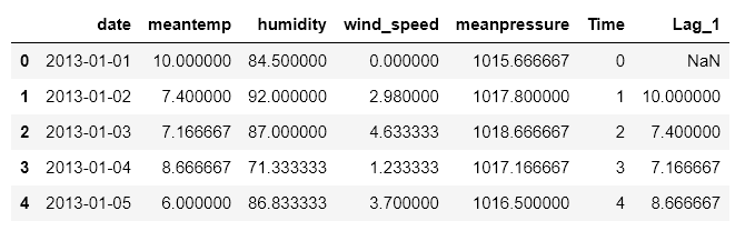

From the above code we have produced a new column with the mean temperature shifted by 1.

We can proceed as before, this time removing our missing value and using Lag_1 as our feature.

# Remove missing values and generate new df
df_lag = df.copy().dropna()

# Training data
X_lag = df_lag[["Lag_1"]]  # feature
y_lag = df_lag.meantemp  # target

# Train the model
model_lag = LinearRegression()
model_lag.fit(X_lag, y_lag)

# Generate a series of predicted values from our lag data
y_lag_pred = pd.Series(model.predict(X_lag))

We can obtain the intercept and coefficient of our model:

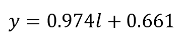
# Obtain model intercept and coefficient
model_lag.intercept_, model_lag.coef_

Leaving us with the model to 3dp:

We can produce a scatter plot of our mean temperature against our lag feature. This can tell us if there exists a correlation between current and previous observations.

plt.figure(figsize=(4, 4))

# Plot the data points
plt.scatter(X_lag, y_lag,label='Actual data')

# Plot the regression line
plt.plot(X_lag, y_lag_pred, color='red', label='Regression line')

# Add labels and a legend
plt.xlabel('Lag_1')
plt.ylabel('Mean Temperature')
plt.title('Simple Linear Regression (Lag feature)')
plt.legend()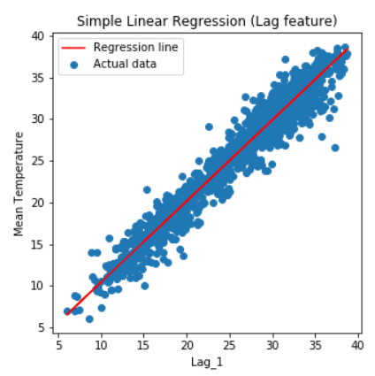

The above plot, shows that an increase in the mean temperature the day before results in an increase in the mean temperature the next day. Correlations such as these indicate it is useful to include a lag feature in the time series model.

Well Built Time Series Models

Well built time series models tend to include a combination of time-step features and lag features. In this episode we used simple linear regression, however we can use such features in other models.

Prev Episode | Next Episode

If you have any questions please leave them below!