
A Gentle Introduction to Time Series Analysis
With video explanation | Data Series | Episode 17.1
Objectives:
- Understand what time series data is and its applications
- Understand the difference between stationary and non-stationary time series
- Be familiar with the different components of time series
- Have an overview of the different techniques used in time series analysis
Before we delve into Time Series Analysis, let us familiarise ourselves with what time series data actually is:
Time Series Overview
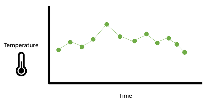
Time Series Definition: An ordered sequence of values of a variable obtained at successive times.
Example: The temperature recorded every two hours during a day would produce a time series.
What we can do with Time Series Data:
- Understand the governing forces and structure that produced the observed data
- Model observed data and make forecasts
General Applications
Some applications of time series analysis include:
- Sales forecasting
- Yield projections
- Workload projections
Components of Time Series
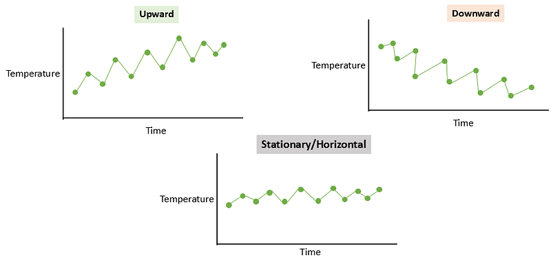
Trend component: The long term-term pattern of a time series.
We can have an upward trend, downward trend and stationary/horizontal trend:
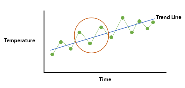
Cyclical component: Up and down movement around the trend line.
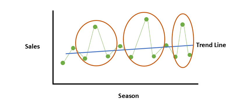
Seasonal Component: Regular fluctuations around the trend line during a fixed interval. This could be during the same season or months every year.
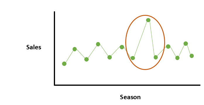
Irregular Component: The unpredictable component. This could be a high fluctuation for example.
Stationary and Non-stationary Time Series
A stationary time series is one whose properties do not depend on the time at which the series is observed. Time series with trends or seasonality are not stationary since the trend and seasonality effects the time series values at different times.
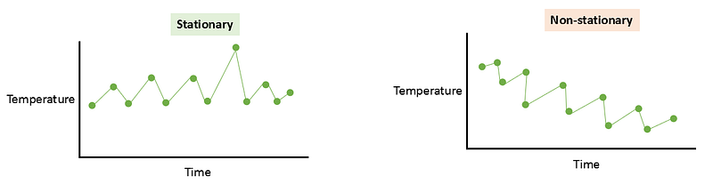
Often, a stationary time series does not have a predictable pattern in the long term.
Time Series Analysis Techniques
Here is an overview of 3 methods used in Time Series analysis.
Traditional Techniques
Moving Average Models: A moving average model uses a regression-like model consisting of past forecast errors for future predictions.

where εₜ is white noise and θ₁ to θq are parameters.
Autoregressive Models: We use a linear combination of past values of the variable to make forecasts.

where εₜ is white noise and ϕ₁ to ϕq are parameters.
Machine Learning Techniques
Machine Learning Models: We can use machine learning regression models like linear regression, LightGBM or a neural network regressor to make predictions on time series data.