
Understanding Simple Linear Regression
Intro to Regression Algorithms | Data series | Episode 4.1
This article is designed to teach the underlying theory of linear regression. How to code and implement this algorithm in Python will be included in episode 4.3. This article also covers some basic Data Science Terminology which is important to know for future episodes.
What is Simple Linear Regression?
Simple Linear regression is a common supervised machine learning algorithm (see episode 3) used by data scientists to make predictions for numerical data such as: future house prices or next year’s sales of a company.
Simple Linear regression should only be used on data where there seems to be a linear relationship between variables. That is our data follows a straight line.
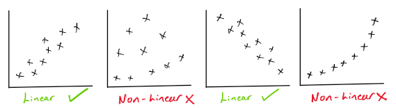
Examples may include house size and house price, or customer reviews and company sales, or height and weight.
The reason why is that simple linear regression relies on a reasonable relationship between variables to make accurate predictions.
Overview
Take a look at the following graph looking at the Temperature and Humidity in Szeged, Hungary.
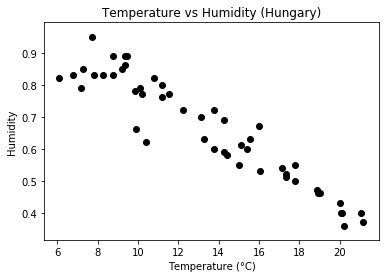

The job of simple linear regression is to find a mathematical relationship between humidity and temperature. It does this by finding whats called “The regression line” which is shown below in blue:
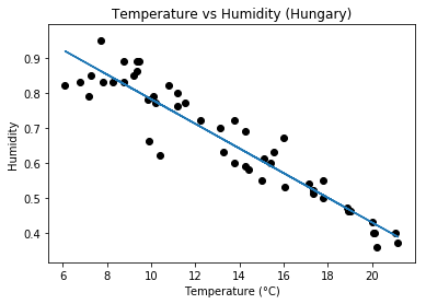
We see that this line gives the general trend of the data that is: As Temperature increases, Humidity decreases. We can then use this line to make predictions for Humidity given any Temperature value.
Because we are using Temperature to predict Humidity: Temperature can be thought of as our input value X and humidity our output y.
Before seeing how this regression line is calculated it is important you are aware of some Data Science Terminology:
Important Data Science Terminology
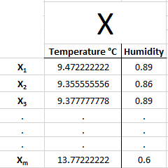
The data we are using to build this regression line is called our training data X. This is the data we use to plot our graph.
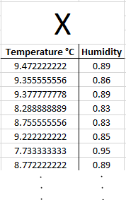
Each training example is called x₁, x₂, x₃, …. ,xₘ , where m in the number of training examples / the last training example:
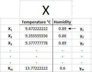
The variable we are trying to predict is humidity, which is called our target value or output y. Each output y is called y₁, y₂, y₃, …. , yₘ:
Calculating the Regression line
The formula of our regression line is be given by:
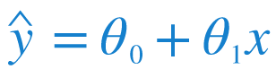
- ŷ is our predicted value for Humidity.
- x is our input Temperature.
- θ₀ and θ₁ are what we call parameters. Changing these parameters change the position of our regression line. So it is these parameters that we are interested in calculating.
The Cost Function
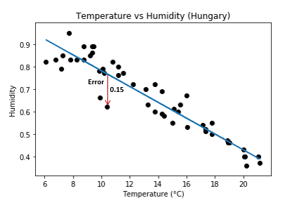
Notice at each point on the graph, there is an “error” between the data point recorded and regression line.
For a temperature of 10.4 °C we got a humidity reading of 0.62
but our regression line predicted a humidity of 0.77 (ŷ).
Our error for this point is given by:
Which is our predicted value minus our actual value.
0.77 - 0.62 =0.15.
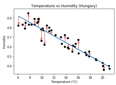
In order to account for all the errors:
We use the following formula. This is called the Cost function:
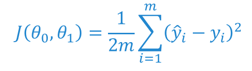
Lets break this down:
- J(θ₀, θ₁) simply states that this is a function and contains the parameters θ₀ and θ₁. ( Remember that ŷᵢ = θ₀ + θ₁𝑥ᵢ ).
- We are essentially squaring all the errors (ŷᵢ - yᵢ), to ensure that they are all positive, and summing them up.
- In order to make the overall error more readable we divide this sum by 2m to give whats called the MSE ( Mean Squared Error ).
To illustrate how this cost is calculated take a look at the following graphs with just three data points.
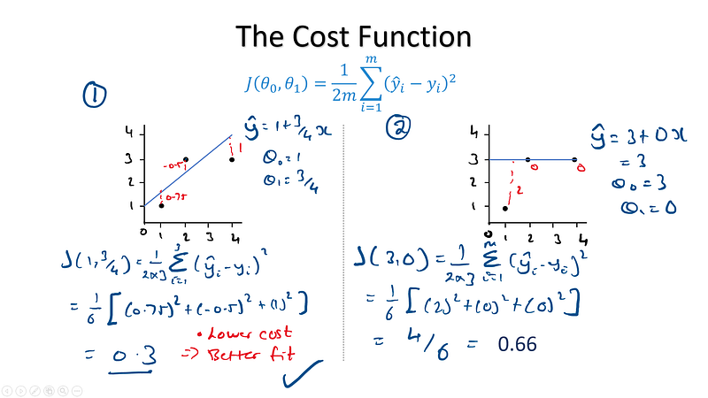
- In case ① we tried a regression line of y = 1+ 3/4𝑥 ,( θ₀ = 1 θ₁ = 3/4) this resulted in a overall cost of 0.3.
- In case ② we tried a regression line of y = 3+ 0𝑥, ( θ₀ = 1 θ₁ = 0) this resulted in a an overall cost of 0.33.
- The first regression line produced a lower cost and therefore is a better fit to the data, but is it the best possible fit?
We want to choose values for θ₀ and θ₁ such that it minimises our cost function. This will result in a regression line y = θ₀ + θ₁𝑥, which fits our data best and therefore produces the most accurate predictions.
Minimising our cost function
Take a look at the following graph which shows how a cost function J(θ₀, θ₁) changes depending on the values of θ₀ and θ₁.
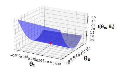
In this case our minimum cost is found at θ₀ = 1.13 and θ₁ = -0.035
Our final most accurate regression line is therefore given by:
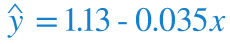
Which is plotted below:
We will then use this formula to predict any future humidity values ŷ given a temperature 𝑥.
The algorithm used to obtain our minimum cost is called Gradient Descent which we will go over in detail in the next episode. [ Episode 4.2 ]
Summary
- Simple Linear Regression is used to find a linear relationship between variables and uses this linear relationship to make future predictions.
- A simple linear regression line is given by ŷ = θ₀ + θ₁𝑥.
- We calculate θ₀ and θ₁ by minimising our cost function using gradient descent.
- We then use this regression line to make future predictions.


