
Understanding Gradient Descent
With video explanation | Data Series | Episode 4.2

This article plans to expand on episode 4.1, explaining Gradient Descent and how it is used to minimise our cost function in Linear Regression. Knowledge of derivatives and partial derivatives will be helpful.
Linear Regression Recap
From the previous episode we calculated the regression line for our humidity and temperature data to be:
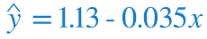
Which we obtained from the cost function graph shown below

The algorithm we use in order to obtain the parameter values that give this minimum cost is called gradient descent.
Overview
The idea of gradient descent is that we start at a random point on our cost function graph, for example here:
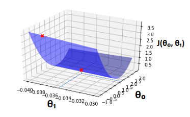
And use partial derivatives in order to obtain make our way down to the minimum.
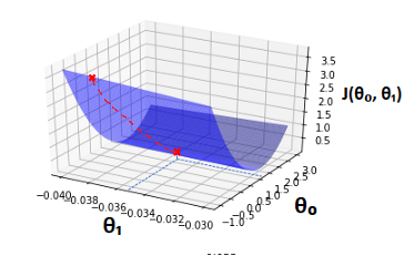
We then look at what parameter values produce this minimum cost and use that in our regression line.
Gradient Descent in 2 Dimensions
Lets take a look at simplified version of gradient descent, with just one parameter θ₁ (where θ₀ = 0), to get the general idea of what is happening.
We plot the cost function J(θ₁) and see how it changes according to θ₁. Please see episode 4.1 to see how this cost function is derived.
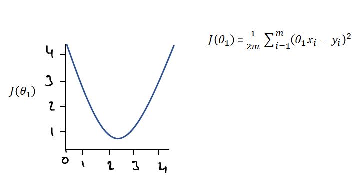
The derivative of our function J(θ₁) is shown in orange.
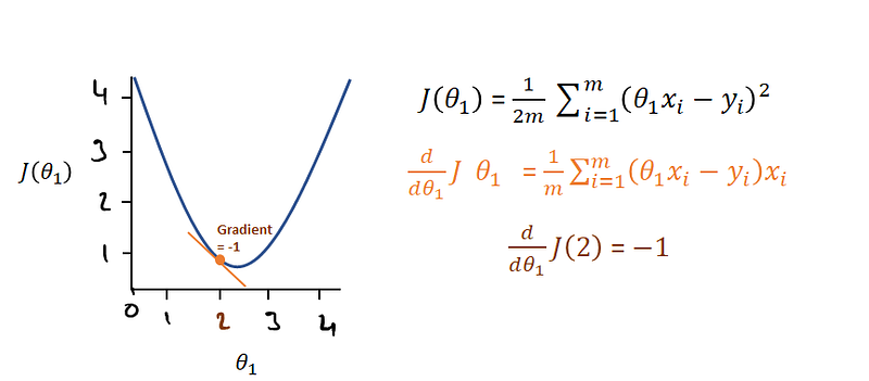
- This essentially gives the slope (or gradient) of our cost function at any value of θ₁.
- For example, as shown in dark orange, at θ₁ = 2, our cost function has a slope of -1.
Gradient Descent Algorithm with 1 parameter
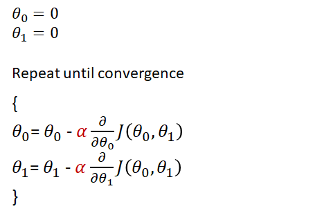
Gradient decent uses our derivative function to reach our minimum cost with the following algorithm.
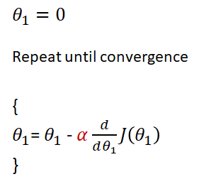
Let’s break this down:
- θ₁ =0 | Initialises our parameter θ₁
- Repeat until convergence| Essentially means repeat until we find a minimum point, this is when d/dθ₁ = 0 and our value of θ₁ remains roughly the same
- We are changing the value of θ₁ upon each iteration by a value of αlpha , which we set ourselves, multiplied by our derivative function d/dθ₁.
- Performing the above operation brings θ₁ closer to our minimum
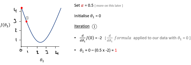
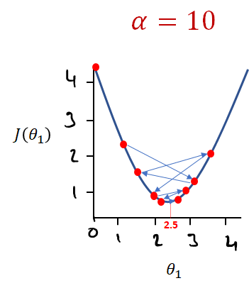
We can apply this algorithm to any shaped cost function to reach our minimum.
Example:
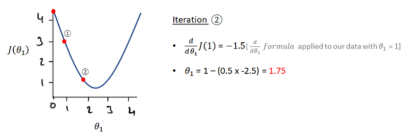
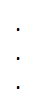
Eventually after n iterations we reach our minimum and we find our optimal value of θ₁ to minimise our cost function as 2.5.
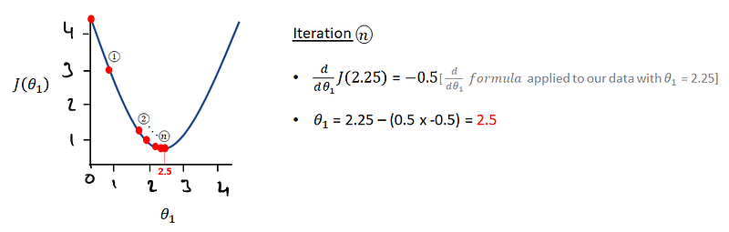
If we try to keep iterating:
Our value for θ₁ remains the same, so we have reached convergence and the algorithm has accomplished its mission.
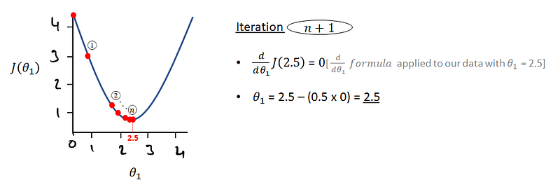
The Learning Rate Alpha ( α )
In the example above we set the learning rate alpha as 0.5. This value determines “how quickly” we approach our minimum.
If Alpha is too small say 0.0001 it may end up taking a very long time to reach our minimum and this takes a lot of computing power. The positive of this, however, is that the minimum value found will be very accurate.
If Alpha is too large say 10 we may end up overshooting and missing our minimum point.
So we compromise by choosing a value of alpha between 0.001 and 1. This in general leads to accurate results fairly quickly with relative little computing power.
One way to choose a good learning rate alpha is by trying values by a scale of 10 so try 0.001 then 0.01 then 0.1 and finally 1 and narrow down a good learning rate which:
a) Reaches minimum cost efficiently
b) Reaches an accurate minimum
Gradient Descent in 3 Dimensions
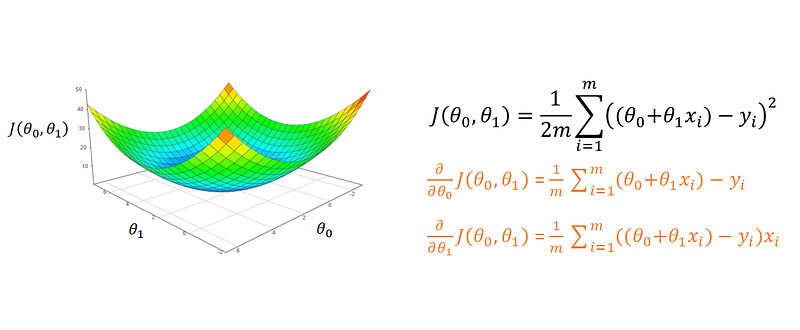
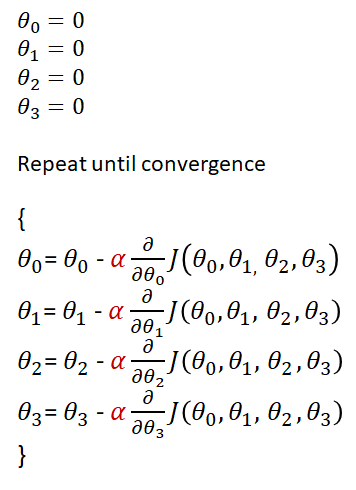
The algorithm for gradient Descent in 3D has the same concept as in 2D but now we are applying the algorithm to both θ₀ and θ₁.
Because we are working in 3 dimensions we have to use whats called partial derivatives to change our values of θ₀ and θ₁ to approach our minimum.
Using the same cost function as in the previous episode the partial derivatives for both θ₀ and θ₁ are given in orange.
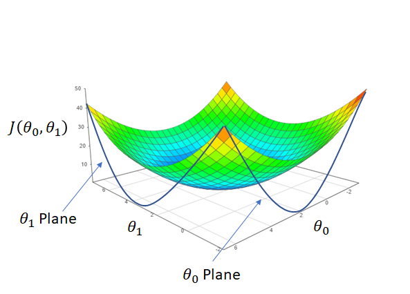
Just as in 2D, the partial derivatives give the slope of the cost function, but this time either in the θ₀ plane or the θ₁ plane:
Gradient Descent Algorithm with 2 parameters
- This algorithm is conceptually the same as gradient descent in 1 dimension.
- We are minimising across the θ₀ plane and the θ₁ shown above to reach our minimum cost.
- In Python we can call a function that does all this maths for us, which i plan to cover in a future episode.
Gradient Descent in multiple Dimensions
Gradient descent in N dimensions often involve more variables, so instead of just one input x trying to be mapped to an output y in 2 dimensions.
With the temperature and humidity example we had the following data and regression line formula.
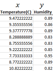
With N dimensions we will be looking to map multiple inputs x to our output temperature, not just humidity but also looking at perhaps pressure and wind speed and seeing how that has an effect on temperature.
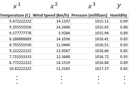
Here each input column is named 𝑥₁,𝑥₂, 𝑥₃ and is assigned its own input parameter θ₁, θ₂ and θ₃ respectively.
It is very difficult to visualise in 4 dimensions, so I won’t be able to show how our cost function changes according to our parameters θ₀, θ₁, θ₂ and θ₃ as shown in 2D and 3D.
The concept remains the same as in 2D and 3D but now we apply the same gradient descent algorithm too all parameters.
Gradient Descent Algorithm with multiple parameters
For n parameters θ₀, θ₁, θ₂, … ,θₙ the algorithm remains the same but we update all n parameters via gradient descent to reach our parameter values that produce our minimum cost.
So for n parameters we have the general gradient descent formula:
Gradient Descent Algorithm for n parameters
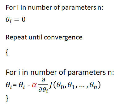
If you can understand both gradient descent in 1 dimension and 2 dimensions don’t worry if n dimensional gradient descent algorithm looks confusing — the computer does all this for us!
I hope you now have a better understanding for gradient descent and what it’s all about and would really appreciate a few claps to keep me going!


