Data Science

Linear Regression Basics for Absolute Beginners

Tutorial on simple and multiple regression analysis using NumPy, Pylab, and Scikit-learn

1. Introduction

Regression models are the most popular machine learning models. Regression models are used for predicting target variables on a continuous scale. Regression models find applications in almost every field of study, and as a result, it is one of the most widely used machine learning models. This article will discuss the basics of linear regression and is intended for beginners in the field of data science.

Using the cruise ship dataset cruise_ship_info.csv, we will demonstrate simple and multiple regression analysis using NumPy, Pylab, and Scikit-learn. Because this is just an introductory tutorial, no distinction between inliers and outliers shall be made (outliers can be handled using more robust methods such as the RANSAC regression).

2. Data Analysis

2.1 Import Necessary Libraries

import numpy as np

import pandas as pd

import pylab

import matplotlib.pyplot as plt

import seaborn as sns

import matplotlib.pyplot as plt

from sklearn.metrics import r2_score

from sklearn.model_selection import train_test_split

from sklearn.preprocessing import StandardScaler

from sklearn.linear_model import LinearRegression

from sklearn.pipeline import Pipeline

pipe_lr = Pipeline([('scl', StandardScaler()),
                    ('lr', LinearRegression())])

2.2 Read dataset and display columns

df = pd.read_csv("cruise_ship_info.csv")

df.head()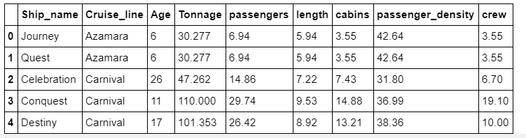

2.3 Calculate the covariance matrix

cols = ['Age', 'Tonnage', 'passengers', 'length', 
                      'cabins','passenger_density','crew']

stdsc = StandardScaler()

X_std = stdsc.fit_transform(df[cols].iloc[:,range(0,7)].values

cov_mat = np.cov(X_std.T)

2.4 Generate a heatmap for visualizing the covariance matrix

plt.figure(figsize=(10,10))sns.set(font_scale=1.5)hm = sns.heatmap(cov_mat,
                 cbar=True,
                 annot=True,
                 square=True,
                 fmt='.2f',
                 annot_kws={'size': 12},
                 yticklabels=cols,
                 xticklabels=cols)
plt.title('Covariance matrix showing correlation coefficients')
plt.tight_layout()
plt.show()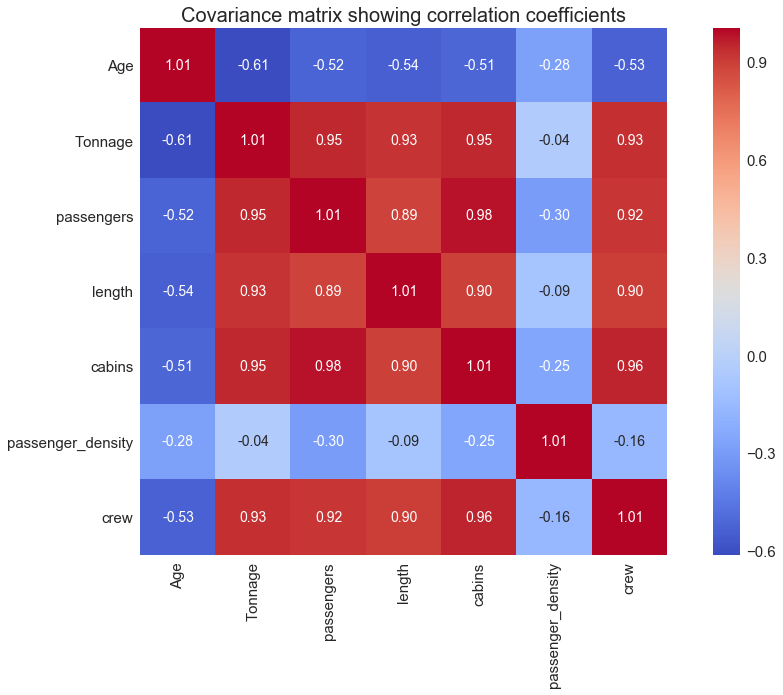

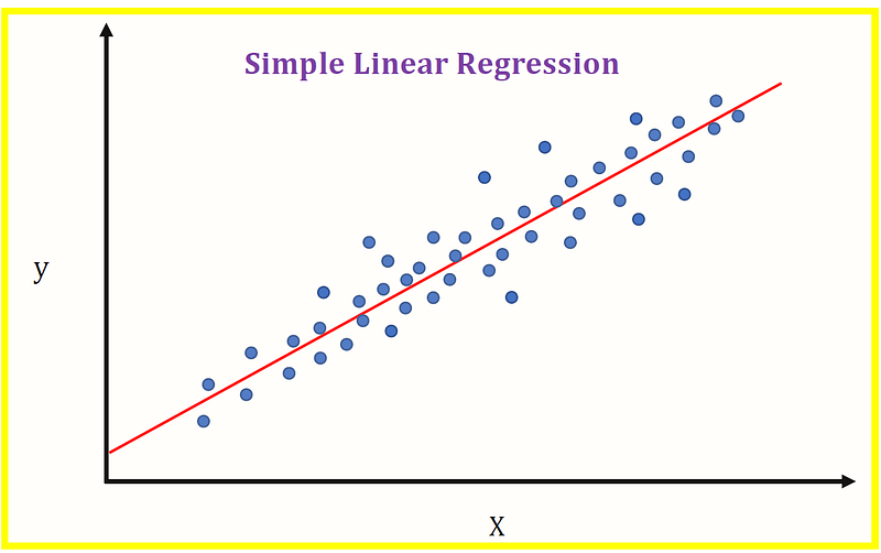
3. Simple Linear Regression

In simple linear regression, there is only one predictor variable. Since our goal is to predict the crew variable, we see from Figure 1 that the cabins variable correlates the most with the crew variable. Hence our simple regression model can be expressed in the form:

where m is the slope or regression coefficient, and c is the intercept. The model will be evaluated using the R2 score metric which can be calculated as follows:

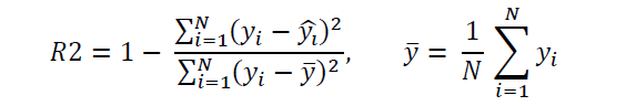
The R2 score takes values between 0 and 1. When R2 is close to 1, it means the predicted values agree closely with the actual values. If R2 is close to zero, then it means the predictive power of the model is very poor.

Let’s now define and plot our independent and dependent variables:

X = df['cabins']

y = df['crew']

plt.scatter(X,y,c='steelblue', edgecolor='white', s=70)

plt.xlabel('cabins')

plt.ylabel('crew')

plt.title('scatter plot of crew vs. cabins')

plt.show()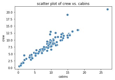

3.1 Simple linear regression using numpy

z = np.polyfit(X,y,1)

p = np.poly1d(z)

print(p)

Output: 0.745 x + 1.216

This shows that the fitted slope is m = 0.745, and the intercept is c = 1.216.

y_pred_numpy = p(X)

R2_numpy = 1 - ((y-y_pred_numpy)**2).sum()/((y-y.mean())**2).sum()

print(R2_numpy)

Output: R2_numpy = 0.9040636287611352

print(r2_score(y, y_pred_numpy))

Output: 0.9040636287611352

Let’s now plot the actual and predicted values:

plt.figure(figsize=(10,7))

plt.scatter(X,y,c='steelblue', edgecolor='white', s=70, 
             label='actual')

plt.plot(X,y_pred_numpy, color='black', lw=2, label='predicted')

plt.xlabel('cabins')

plt.ylabel('crew')

plt.title('actual and fitted plots')

plt.legend()

plt.show()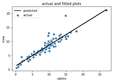

3.2 Simple linear regression using Pylab

degree = 1

model= pylab.polyfit(X,y,degree)

print(model)

Output: array([0.7449974 , 1.21585013]). We see again that the slope is m = 0.745, and the intercept is c = 1.216.

y_pred_pylab = pylab.polyval(model,X)

R2_pylab = 1 - ((y-y_pred_pylab)**2).sum()/((y-y.mean())**2).sum()

print(R2_pylab)

Output: R2_pylab = 0.9040636287611352

print(r2_score(y, y_pred_pylab))

Output: 0.9040636287611352

3.3 Simple linear regression using scikit-learn

lr = LinearRegression()

lr.fit(X.values.reshape(-1,1),y)

print(lr.coef_)

print(lr.intercept_)

Output: [0.7449974], 1.2158501299368671. We see again that the slope is m = 0.745, and the intercept is c = 1.216.

y_pred_sklearn = lr.predict(X.values.reshape(-1,1))

R2_sklearn = 1 - ((y-y_pred_sklearn)**2).sum()/((y-y.mean())**2).sum()

print(R2_sklearn)

Output: R2_sklearn = 0.9040636287611352

print(r2_score(y, y_pred_sklearn))

Output: 0.9040636287611352

We observe that all 3 methods for basic linear regression (NumPy, Pylab, and Scikit-learn) gave consistent results.

4. Multiple Linear Regression with Scikit-Learn

From the covariance matrix plot above (Figure 1), we see that the “crew” variable correlates strongly (correlation coefficient ≥ 0.6) with 4 predictor variables: “Tonnage”, “passengers”, “length, and “cabins”. We can, therefore, build a multiple regression model of the form:

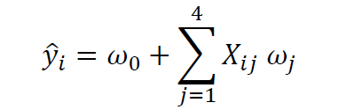
where X is the features matrix, w_0 is the intercept, and w_1, w_2, w_3, and w_4 are the regression coefficients.

4.1 Define features matrix and the target variable

cols_selected = ['Tonnage', 'passengers', 'length', 'cabins','crew']

df[cols_selected].head()

X = df[cols_selected].iloc[:,0:4].values    # features matrix 

y = df[cols_selected]['crew'].values        # target variable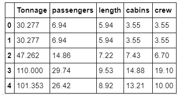

4.2 Model building and evaluation

X_train, X_test, y_train, y_test = train_test_split( X, y, test_size=0.3, random_state=0)

sc_y = StandardScaler()

y_train_std = sc_y.fit_transform(y_train[:,np.newaxis]).flatten()

pipe_lr.fit(X_train, y_train_std)

y_train_pred = sc_y.inverse_transform(pipe_lr.predict(X_train))

y_test_pred = sc_y.inverse_transform(pipe_lr.predict(X_test))

r2_score_train = r2_score(y_train, y_train_pred)

r2_score_test = r2_score(y_test, y_test_pred)

print('R2 train for lr: %.3f' % r2_score_train)

print('R2 test for lr:  %.3f ' % r2_score_test)

Output:

R2 train for lr: 0.912 R2 test for lr: 0.958

4.3 Plot the output

plt.scatter(y_train, y_train_pred, c='steelblue', edgecolor='white', s=70, label='fitted')

plt.plot(y_train, y_train, c = 'red', lw = 2,label='ideal')

plt.xlabel('actual crew')

plt.ylabel('predicted crew')

plt.legend()

plt.show()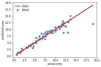

5. Summary

In summary, we’ve presented a tutorial on simple and multiple regression analysis using different libraries such as NumPy, Pylab, and Scikit-learn. Linear regression is the most popular machine learning algorithm. A thorough understanding of linear regression would serve as a good foundation for understanding other machine learning algorithms such as logistic regression, K-nearest neighbor, and support vector machine.

Additional Data Science/Machine Learning Resources

Data Science Minimum: 10 Essential Skills You Need to Know to Start Doing Data Science

Data Science Curriculum

Essential Maths Skills for Machine Learning

3 Best Data Science MOOC Specializations

5 Best Degrees for Getting into Data Science

5 reasons why you should begin your data science journey in 2020

Theoretical Foundations of Data Science — Should I Care or Simply Focus on Hands-on Skills?

Machine Learning Project Planning

How to Organize Your Data Science Project

Productivity Tools for Large-scale Data Science Projects

A Data Science Portfolio is More Valuable than a Resume

Data Science 101 — A Short Course on Medium Platform with R and Python Code Included

For questions and inquiries, please email me: [email protected]