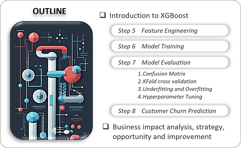
Customer Churn Prediction — 8 Steps For Building XG Boost Model Part 2 — Model Training, Evaluation, Prediction, and Interpretation

Customer churn, which occurs when customers stop doing business with a company, can have significant financial implications for businesses. Using machine learning, we can effectively identifying patterns and characteristics of customers likely to churn. By proactively addressing these insights, businesses can strategise retention efforts, ensuring sustained customer engagement and loyalty. Let’s first familiarise ourselves with the core principles and characteristics of XGBoost.

Introduction to XGBoost

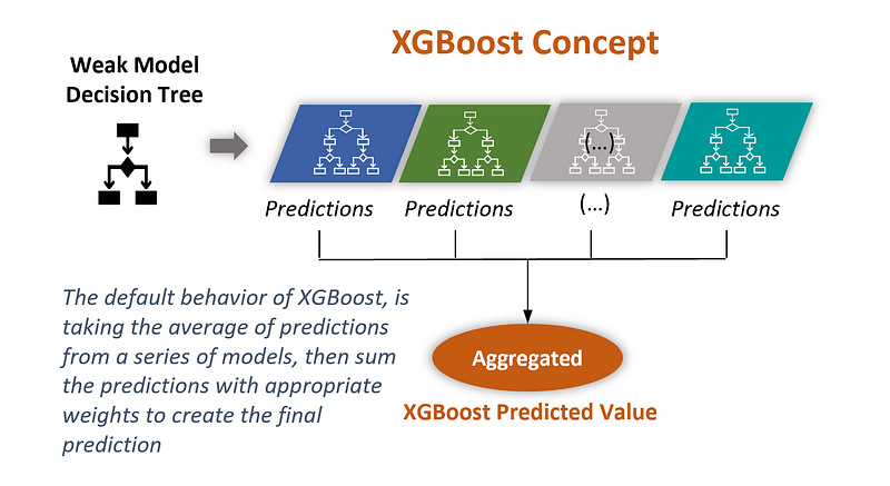
XGBoost, short for eXtreme Gradient Boosting, is a powerful machine learning algorithm renowned for its efficiency and accuracy. It belongs to the family of gradient boosting algorithms, which combine the predictions of multiple weak models (typically decision trees) to create a strong predictive model.

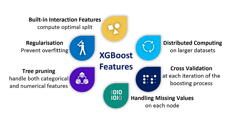
XGBoost incorporates several enhancements over traditional gradient boosting algorithms, making it highly efficient and effective. Some notable features of XGBoost include.

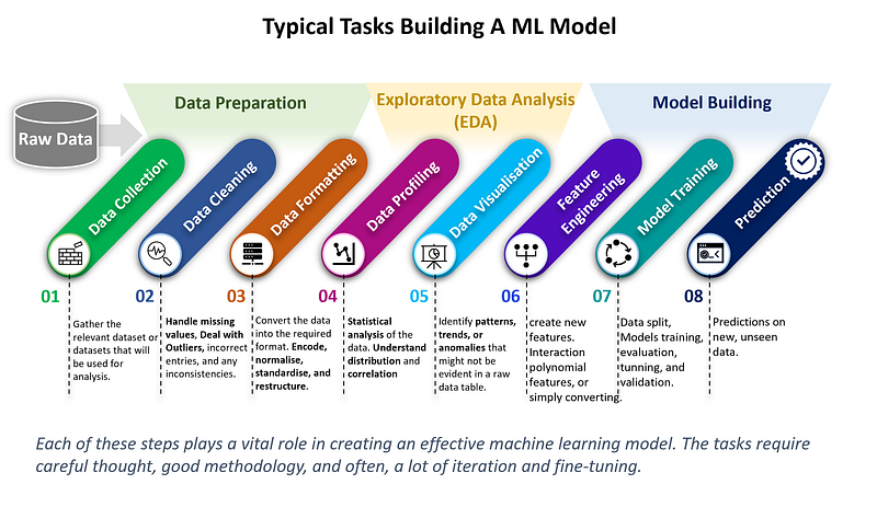
In Part 1 of the tutorial, I laid out a common path for constructing a machine learning model. This process illustrates the three key stages involved. First, there’s the preparation of the data, ensuring it’s in the right format. Next, Exploratory Data Analysis (EDA) helps us understand the patterns within. Finally, it delves into model building, where the magic really happens, turning data into predictive power.

Summary — Building XGBoost Model Part 1

In Part 1, we delved deep into Exploratory Data Analysis (EDA) as a crucial step in building an ML model.

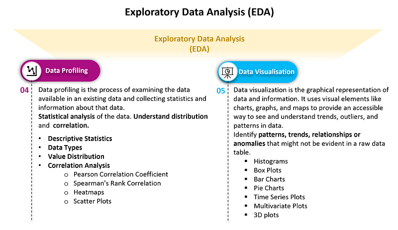
It provided an understanding of our customer churn dataset, detailing each step of data preparation, profiling, correlation analysis, and visualization. Various insights are drawn from the visualizations to understand customer behavior and preferences that lead to churn.

Specific EDA Analysis and Insights

Data Preparation and Profiling: The EDA begins with cleaning the Telco customer dataset, handling missing values, dealing with outliers, and addressing imbalanced datasets. Descriptive statistics provide an understanding of customer tenure, monthly charges, and the total amount charged.

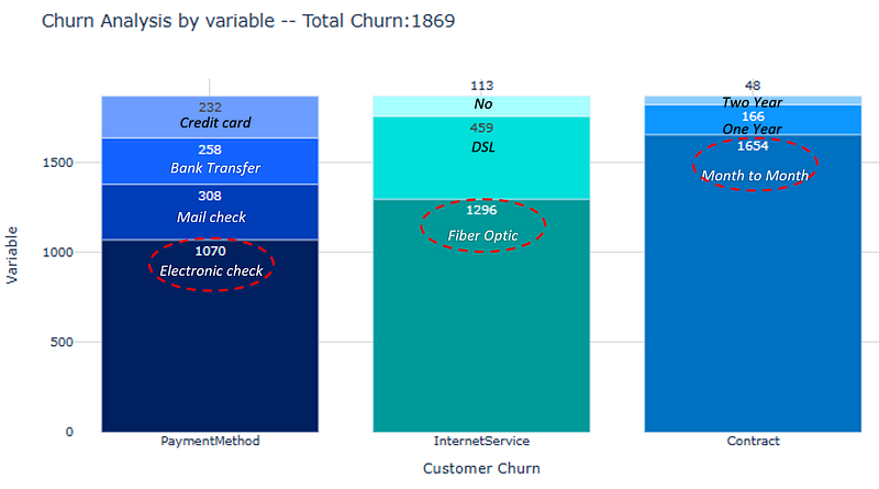
Correlation Analysis: Correlation matrices are used to find the top features influencing churn, such as contract type, internet service, and payment method.

Contract Type: A strong correlation was found between the type of contract and churn. Customers with month-to-month contracts were significantly more likely to churn. This indicates that short-term contracts might not foster customer loyalty as effectively as longer-term contracts.
Internet Service: The type of internet service was highly correlated with churn, especially fiber optic connections. Customers with fiber optic service were more likely to churn, possibly due to higher costs or expectations. Conversely, those without internet service had the lowest churn rates, suggesting satisfaction with basic or no-internet packages.
Payment Method: The method of payment, particularly electronic checks, was identified as having a correlation with higher churn rates. This could indicate dissatisfaction with this payment method or reflect a broader demographic that prefers electronic checks and is more prone to churn.

Techniques like One-Hot and Ordinal Encoding transform categorical features, and multicollinearity is detected and managed.

Visualization Insights: Various visualizations reveal key churn trends and patterns:

The combination of statistical analysis and visualizations in EDA provides a comprehensive understanding of the factors that drive churn. These specific insights provide a multifaceted view of customer churn and highlight key areas where interventions could be targeted. Understanding the correlations and visual patterns helps in crafting data-driven strategies to address churn, such as offering special packages for incentivizing longer-term contracts or improving payment methods. These insights are valuable for both strategic decision-making and model building in predicting and mitigating customer churn.

Model development

Now, let’s transition into the XGBoost model development phase, including feature engineering, model training, evaluation, prediction, and interpretation.

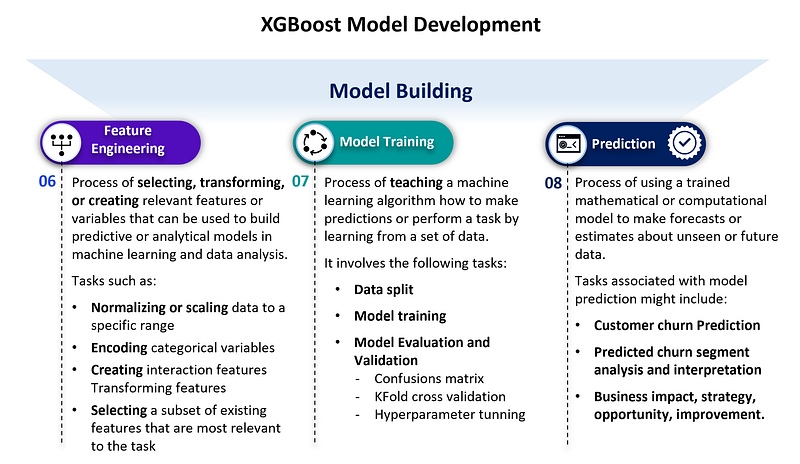
Step 5: Feature Engineering

Following Step 4, “Data Visualization,” in Part 1 of the article, we are now ready to delve into the next phase of our analysis: Feature engineering.

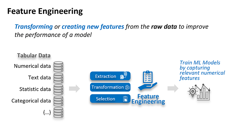
Feature engineering is the process of using domain knowledge to extract features (characteristics, properties, attributes) from raw data. It involves transforming or creating new variables to better represent the underlying patterns in the data. By highlighting essential aspects and relationships, feature engineering can significantly enhance the performance of machine learning models.

Normalize and Encode Data

This step ensures that our dataset is in the optimal format for machine learning algorithms, paving the way for more advanced analysis and modelling. Let’s explore how to effectively normalize and encode our data to prepare for the subsequent stages of our customer churn prediction process.

Feature Scaling

Many machine learning algorithms are sensitive to features being on different scales, such as metric-based algorithms (e.g., KNN, K-Means) and gradient descent-based algorithms (e.g., regression, neural networks). Feature scaling is performed to normalize or standardize the range or distribution of features in a dataset. This process is necessary for certain machine learning algorithms to ensure fair comparisons and prevent features with larger magnitudes from dominating the learning process. Some of solutions for feature scaling:

Min-Max Scaling (Normalization): Rescales features to a specific range, often between 0 and 1, preserving the original distribution.
Standardization: Transforms features to have zero mean and unit variance. It maintains the shape of the distribution but makes the data more interpretable and suitable for algorithms that assume normality.
Log Transformation: Applies a logarithmic function to reduce the scale of highly skewed features.

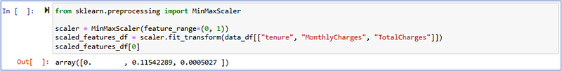
In this analysis, I’ve used Min-Max Scaling to rescale features between 0 and 1. This essential step ensures fair comparisons among features, enhancing the machine learning model’s performance.

Just as in Part 1, here we use Jupyter Notebook to write Python code in this session. If you need common shortcuts reference within Jupyter Notebook you’ll find a detailed guide for your reference in Part1.

We won’t need it for our XGBoost example but here is the code snippet if you ever need it.

Feature Extraction

e.g. date -> week day, month, year, season.

We don’t have dates in the dataset but the customerID has 2 parts that could potentially have a meaning and might be worth extracting. Let’s check!

Create 2 new columns with each parts of the ID.

Check the cardinality of each feature.

Although it is worth investigating, having high cardinality in a feature does not necessarily indicate its usefulness in distinguishing between two records. Therefore, in this case, we will disregard the high cardinality feature and remove the customerID from the dataset.

Feature Building/Construction

‘Binning age’ can enhance the robustness of certain models, reducing overfitting, but it comes at the cost of losing information due to the tradeoff involved.

What can a human interpret from looking at the data that an algorithm wouldn’t be able to see?

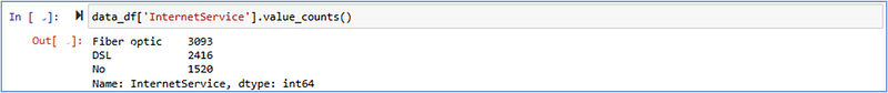
Humans are aware of the speed difference between Fiber optic and DSL internet services, but an algorithm would not be able to infer that from the column alone. To address this, the suggestion is made to assign a numerical representation to the categories that represents their speed on a scale. Specifically, assigning 0 to ‘No’, 10 to ‘DSL’, and 150 to ‘Fiber’ as speed indicators.

Feature Selection

Feature selection is the process of reducing the number of input variables when developing a predictive model. It is desirable to reduce the number of input variables to both reduce the computational cost of modelling and, in some cases, to improve the performance of the model. Indeed, the performance of some models can degrade when including input variables that are not relevant to the target variable.

Do you remember our correlation matrix in Part 1? Let’s use it again to identify the feature-feature linear dependency and if one is very high that will mean that we can probably drop on of them as they will be redundant to our model.

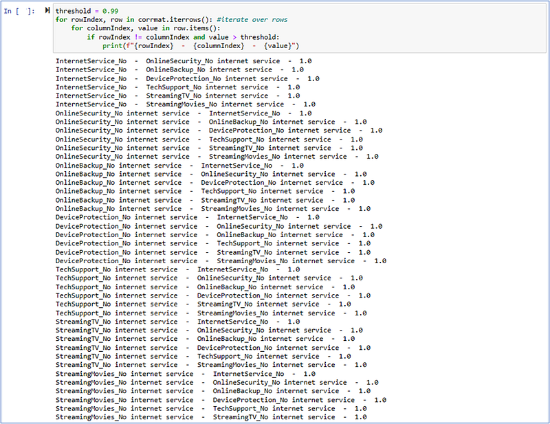
The code is iterating over a correlation matrix (corrmat) and printing out pairs of strongly correlated features based on a given threshold (0.99).

The code checks each pair of features in the correlation matrix that have a correlation coefficient greater than the threshold value (0.99).
For each pair of correlated features, it prints the names of the features (rowIndex and columnIndex) and their corresponding correlation value (value).

The result indicates that there are six pairs of strongly correlated features, all directly related to the feature “InternetService_No”. The pairs have a correlation coefficient of 1.0, indicating a perfect positive correlation.

This means that if a customer does not have internet service (InternetService_No), they are also highly likely to have no internet-related features like online security, online backup, device protection, tech support, streaming TV, and streaming movies.

These correlations suggest that the presence or absence of internet service is strongly associated with these specific features, indicating that customers without internet service tend to have these other services disabled or not subscribed to. This insight can be valuable in understanding the relationship between different features and their impact on customer churn.

Encoding Categorical Features

As explained the encoding categorical features in Part 1 Step 3, we will now proceed to encode the Data_df dataset in preparation for model development.

Encoding categorical features is a crucial step in preparing data for machine learning models. Categorical features are variables that take on discrete values.

Step 6: Model Training

In machine learning, it is common to divide the available data into different datasets for various purposes. Here’s an overview of the typical datasets used in the training, validation, and testing stages.

Data split

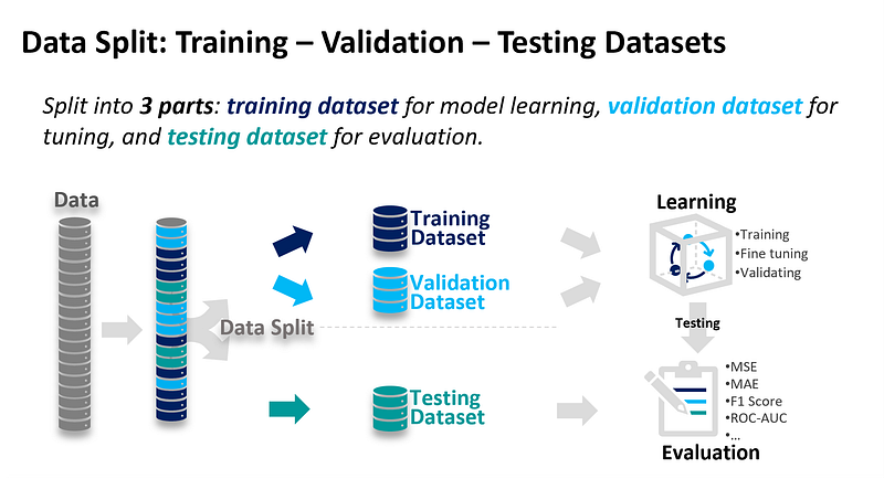
It is crucial to ensure that these datasets are independent and representative of the underlying data distribution. Random sampling or techniques like cross-validation can be employed to create these datasets. Furthermore, it is important to refrain from using the testing dataset during any training or tuning process to avoid biased evaluation.

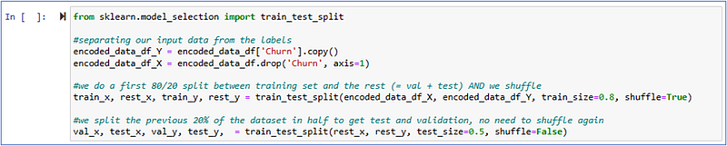
Let’s use a sklearn function for the split and do not forget shuffling your data before splitting to make sure your observations are evenly distributed across train and test.

We aim at doing a 80/10/10 for our train/validation/test sets.

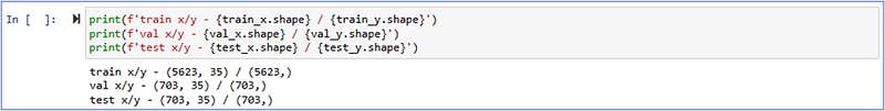
The output confirms the successful splitting of the data into training, validation, and test sets based on the specified proportions. The data is now ready for further analysis, model training, and evaluation.

XGBoost and Decision Trees

Xgboost, a very popular algorithm for classifying tabular data, utilises decision trees and ensemble models, employing both bagging and boosting techniques.

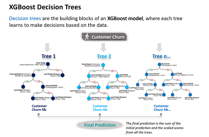
Explanation of tree n…:

Root Node: The tree begins by evaluating whether the customer has Tech Support. Based on this condition, the data is split into two branches.
Internal Nodes: These nodes further refine the data by evaluating conditions on features like MultipleLines, tenure, StreamingMovies, and PhoneService.
Leaf Nodes: These are the final decisions about customer churn (Churn = Yes or Churn = No), based on the conditions in the preceding nodes.

Again, this is just a hypothetical example. The power of XGBoost comes from the way it combines the predictions of many simple trees. By focusing each tree on correcting the errors of the previous trees, and by learning gradually through the use of a learning rate, XGBoost can achieve high accuracy without overfitting the training data.

Mathematically, the final prediction for a given instance can be represented as:

where η is the learning rate, n is the number of trees, and the score of tree i is the score for the given instance from the i-th tree.

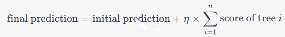
Training your model with XGBoost

Classifier configuration:

Objective: “binary:logistic”, appropriate for binary classification, use ‘multi:softprob’ for multiclass problems.
Random_state: to ensure consistent results across training rounds.
N_estimators: the number of sub-trees used.
Max_depth: the maximum number of splits in sub-trees.
Min_child_weight: a threshold to stop splitting when leaf sample size falls below it.
Learning_rate: to shrink feature weights for a conservative boosting process.
Scale_pos_weight: helps in handling unbalanced datasets by focusing more on positive observations.

Fit method notes:

eval_metric=”aucpr” (area under the curve precision recall)
early_stopping_rounds: if no improvement is recorded after 10 rounds of tree creation then stop

We generate predictions for the train dataset to see how it fitted the training data.

We generate predictions for the test dataset.

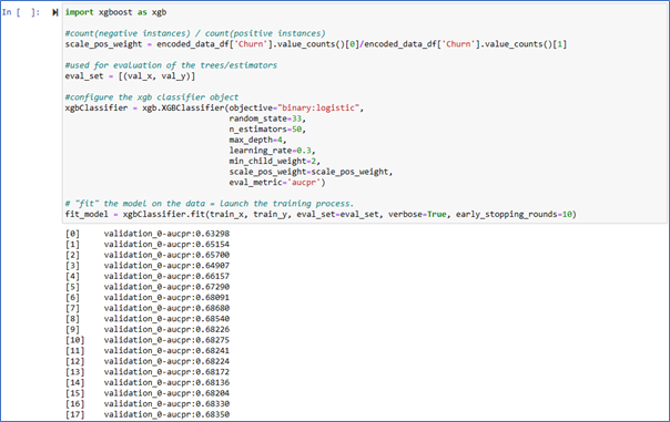
Step 7: Model Evaluation

Feature Importance/Weight

You can use plot important to understand which features are especially important. By default, this method calculate “importance” based on the” weight”. The weight is the number of times a feature appears in a tree.

Visual Representation of your trees

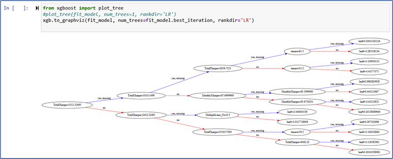
Note that the final probability prediction is obtained by taking sum of leaf values (raw scores) in all the trees and then transforming it between 0 and 1 using a sigmoid function. The leaf value (raw score) can be negative, the value 0 actually represents probability being 1/2.

1. Confusion Matrix

It’s especially useful for binary classification problems (classifying items into one of two classes) but can be extended to multi-class problems as well. It is the best way to evaluate the performance of a classifier model.

Here’s what a confusion matrix looks like for binary classification — example of illustration:

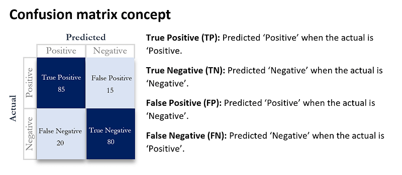
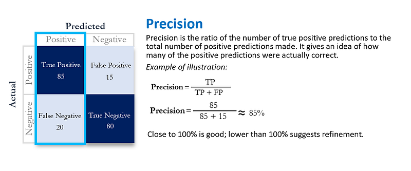
Below are some of the key classification metrics derived from the confusion matrix, along with explanations for each:

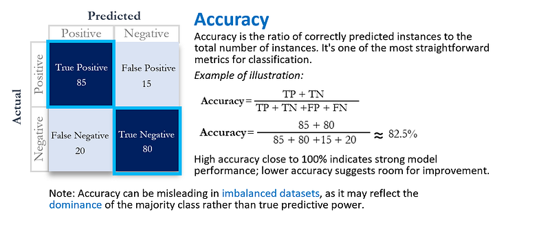
These metrics provide different perspectives on the model’s performance, allowing for a more comprehensive evaluation.

Let’s implement them with the customer churn data.

Set up the confusion matrix for the test dataset.

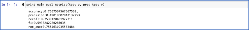
Below are the main metrics for the test dataset.

Choosing the right evaluation metric depends on the specific problem, the business context, and the nature of the data.

Accuracy: Use when classes are balanced; avoid if imbalanced. Measures overall correctness.
Precision: Crucial when minimizing false positives is key, e.g., spam email detection.
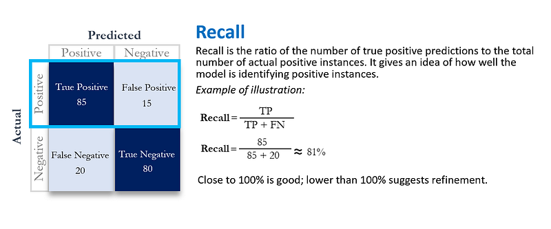
Recall (Sensitivity): Essential when minimizing false negatives, e.g., medical diagnosis.
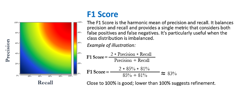
F1 Score: Balances precision and recall, useful in fraud detection.
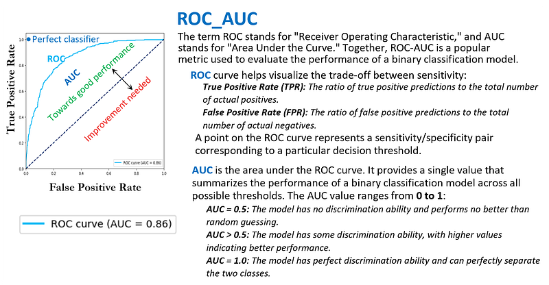
ROC AUC: Evaluates ability to distinguish classes; avoid if highly imbalanced, e.g., credit approval.

TIPS:

Imbalanced Dataset: Consider using Precision, Recall, F1 Score, or a custom metric tailored to the specific business cost of errors.
Threshold-Independent Evaluation: Use ROC AUC to evaluate the model’s ranking ability.
Custom Business Objectives: Consider developing a custom metric that directly aligns with the business objective or cost function.

For customer churn prediction: the focus should primarily be on Recall, as not predicting that a customer will churn is a big miss and can lead to loss of revenue and customer relationship. On the other hand, predicting that a customer might churn while they do not will just trigger specific retention campaigns that might be unnecessary but are generally less harmful.

In this context, a false negative (failing to identify a churning customer) is more costly than a false positive (incorrectly identifying a non-churning customer). Therefore, optimizing for Recall ensures that the model catches as many actual churn cases as possible, even if it means occasionally targeting non-churning customers with retention efforts. The use of F1 Score can also be considered to balance Precision and Recall if the cost of false positives becomes significant, but the primary emphasis should remain on Recall.

Confusion Matrix Metrics:

Accuracy (75.68%): This shows that the model correctly predicts both churn and retention approximately 75.68% of the time. It’s a general measure of how often the model is correct.
Precision (49.02%): This is a measure of how many of the predicted churns were actually churns. A precision of 49.02% means that out of all the customers the model predicted would churn, only about 49.02% actually did. This could mean that the model is over-predicting churn.
Recall (75.30%): This metric tells us how many of the actual churns were correctly identified by the model. A recall of 75.30% means that the model identified 75.30% of all actual churn instances. It is focused more on minimizing the false negatives.
F1 Score (59.38%): The F1 score is the harmonic mean of precision and recall, giving a balanced view of the model’s performance. An F1 score of 59.38% indicates that the model may need improvement in achieving a balance between precision and recall.
ROC AUC (75.55%): The ROC AUC score provides an aggregate measure of performance across all possible classification thresholds. A value of 75.55% indicates that the model has a good ability to distinguish between customers who will churn and those who will not.

2. KFold Cross-Validation

It is a resampling procedure used to evaluate machine learning models on a limited data sample. It provides a more robust assessment of a model’s performance by reducing the variance associated with a single random train-test split.

Here’s how KFold cross-validation works:

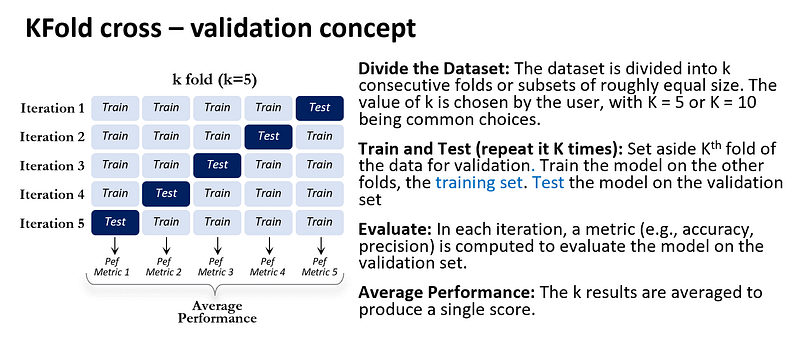
KFold cross validation uses different splits, it provides a more generalized performance estimate. All observations are used for both training and validation (to be tested), ensuring that the evaluation is not overly dependent on the particular split of data. However, it requires training and evaluating the model k times, increasing computational cost and If the data is not shuffled properly, the folds might be biased.

Let’s implement the KFold cross-validation concept by utilizing confusion matrix metrics with our customer churn data.

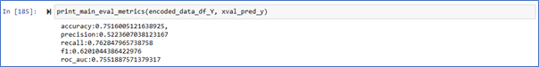
Precision is slightly higher in the KFold method, indicating better identification of true positives among the predicted positives. The recall is also slightly higher in the KFold cross-validation, reflecting better identification of all relevant instances. The F1 score, a balance between precision and recall, is slightly higher in the KFold method, suggesting a more harmonized trade-off between these two metrics in the cross-validated approach.

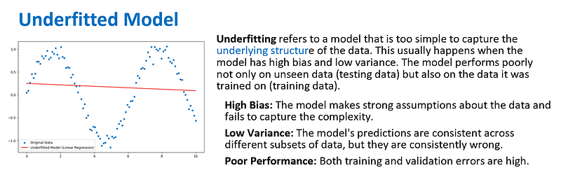
3. Intuition about Underfitting and Overfitting

Model evaluation in machine learning involves assessing how well a model’s predictions match the true outcomes. Three common scenarios that arise during this evaluation are underfitting, overfitting, and achieving a good fit.

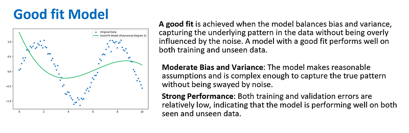
The process of model selection and tuning often involves finding the right balance between underfitting and overfitting, aiming for a model that achieves a good fit with the data while able to generalize. Techniques like cross-validation, regularization, and early stopping can help in this process.

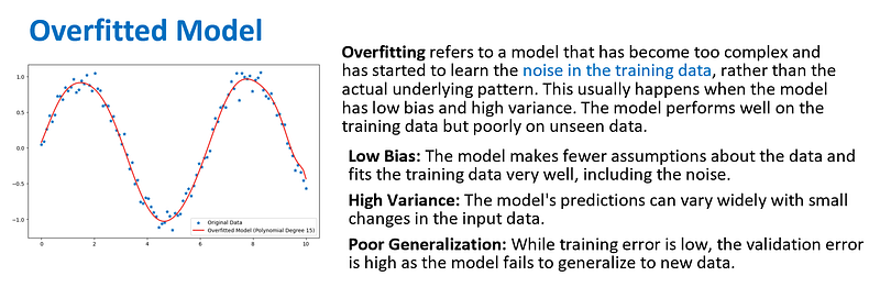
Overfitted Model Example:

Let’s generate an overfitted model as an example.

We generate predictions on both the train and test set.

Evaluation metrics on the training dataset.

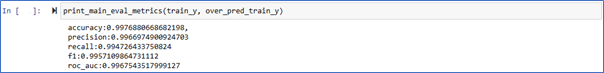
The performance above on the training data is nearly perfect, with extremely high values for all metrics. This indicates that the model has almost flawlessly learned the training data, including its noise and specific details.

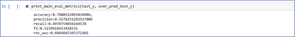
Evaluation metrics on the test dataset below. In contrast, the performance on the test data (unseen data) is significantly lower. All metrics are notably reduced compared to the training performance, with precision, recall, and F1 score being especially affected.

Interpretation:

High Discrepancy: The large discrepancy between training and test performance is a strong sign of overfitting. The model has become too specialized to the training data and fails to generalize well to new, unseen data.
Implications for Customer Churn: In a customer churn context, overfitting can lead to unreliable predictions for real-world customers. The model’s ability to identify customers at risk of churning is compromised, as seen in the lower recall on the test set (49.40%).
Potential Consequences: Overfitting can lead to misguided business decisions, such as targeting the wrong customers with retention campaigns or missing opportunities to retain customers who are likely to churn.

Implementing regularization techniques may prevent the model from fitting the noise in the training data.

Quick Explanation of Regularization

Regularization is a technique used to prevent overfitting by keeping a model’s parameters or weights “in check” and not too large. For example, “L2” regularisation applies a penalty to the quality metrics, forcing the algorithm to keep weights relatively small. In tree-based methods, it may limit the number of splits by defining a minimum gain or using other constraints. By constraining the complexity of the model, regularization helps to ensure that the model generalizes well to unseen data.

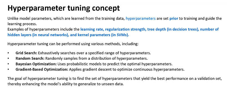
4. Hyperparameter Tuning

Hyperparameter tuning is the process of systematically searching for the best combination of hyperparameters that maximize the performance of a machine learning algorithm.

Let’s configure the hyperparameters for our model as an example.

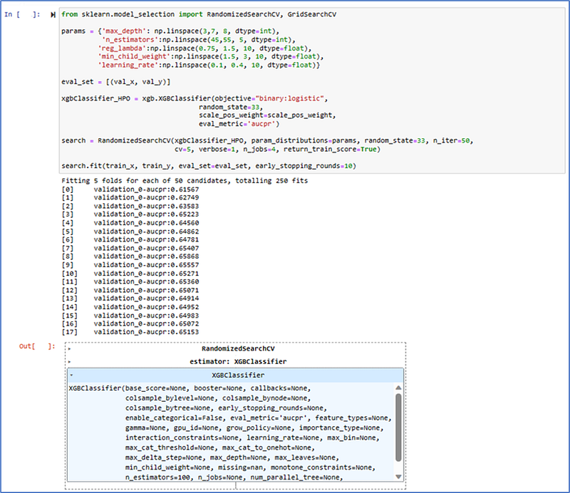
The given code snippet is performing hyperparameter tuning for an XGBoost classifier using randomized search cross-validation. Here’s a detailed explanation of each part:

The code provided sets up hyperparameter tuning for the XGBoost classifier, focusing on optimizing hyperparameters related to model complexity, regularization, and learning. Here’s a detailed breakdown of each part:

RandomizedSearchCV: Hyperparameter tuning by random sampling, more efficient for large hyperparameter spaces.
Hyperparameter Grid: Includes parameters like ‘max_depth’ (3 to 10), ‘n_estimators’ (10 to 50), ‘reg_lambda’, ‘min_child_weight’, ‘learning_rate’ (0.2 to 0.4) for model tuning.
Validation Set: Used for early stopping if no improvement for 10 consecutive rounds.
XGBoost Classifier: Binary classification with ‘objective=”binary:logistic”’, reproducibility, imbalance handling, ‘eval_metric=’aucpr’’.
Randomized Hyperparameter Search: 50 iterations, 5-fold cross-validation, parallel processing with 4 CPU cores.
Model Fitting: With early stopping on validation set.

Overall, this code snippet efficiently explores a wide range of hyperparameters to find a robust and well-fitted XGBoost model for binary classification, targeting customer churn prediction.

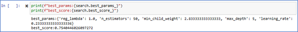
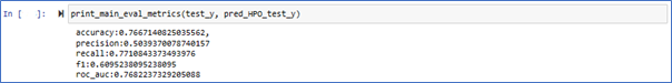
Hyperparameter optimization (HPO) has led to a slight improvement in the model’s performance across all key metrics. Overall, the first set of parameters used was already “manually” tuned so we don’t see a massive difference though the accuracy, precision, recall, F1 score, and ROC AUC values have all increased after tuning, indicating a more fine-tuned prediction capability. Specifically, the recall has seen improvement, demonstrating the model’s enhanced ability to correctly identify customers who are at risk of churning.

Step 8: Customer Churn Prediction and Interpretation

Churn Prediction and Interpretation

Let’s use the best-fit model, identified through hyperparameter tuning, to predict the number of customer churns. This approach ensures that we are employing the most optimized and finely-tuned model for accurate predictions.

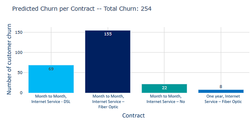
The prediction on the test set indicates that 254 customers are predicted to churn. Here’s a detailed interpretation focused on customer churn analysis, including business impacts and recommendations:

Interpretation of Customer Churn Prediction

The prediction of 254 customers likely to churn in the test set could be influenced by various factors. Analyzing the segments previously described gives us insights into why this churn might be happening:

Contract Type: Month-to-month contracts are more common among those predicted to churn. This flexibility might lead to higher churn rates.
Internet Service: Different types of internet services (DSL, Fiber optic, No Internet) have shown varied churn behaviors.
Tenure: Shorter tenure in some segments indicates dissatisfaction, while longer tenure shows commitment.
Proportion of Senior Citizens: Varied proportions of senior citizens across segments might influence churn patterns.

Business Impacts

Revenue Loss: Losing 254 customers can lead to significant revenue loss, especially if they belong to high-value segments like Fiber optic.
Brand Reputation: High churn rates can negatively impact brand reputation and customer loyalty.
Opportunity Costs: Losing customers to competitors might mean losing opportunities for upselling or cross-selling other products or services.

Business Improvement Recommendations

Enhance Customer Engagement: Implement personalized engagement strategies to understand customer needs and preferences.
Offer Incentives for Long-Term Contracts: Provide discounts or value-added services for customers willing to commit to longer-term contracts.
Improve Service Quality: Regularly monitor and enhance the quality of internet services to ensure customer satisfaction.
Churn Prevention Programs: Implement proactive churn prevention programs by identifying at-risk customers early and providing targeted interventions.

Model Improvement Opportunities

Feature Engineering: Create and include more features that reflect customer behavior, satisfaction levels, and engagement with various services.
Hyperparameter Tuning: Regularly update and optimize the model’s hyperparameters to reflect the changing customer base and market conditions.
Use Ensemble Methods: Combining different predictive models might improve accuracy in predicting churn.
Customer Segmentation: Apply advanced clustering or segmentation techniques to identify nuanced customer behaviors that might lead to churn.
Regular Model Evaluation: Continuously evaluate the model’s performance on new data and make necessary adjustments to ensure its relevance and accuracy.

The prediction of 254 customers churning represents a critical challenge and opportunity for the business. Understanding the underlying factors through detailed segmentation, coupled with strategic interventions and continuous model improvements, can turn this challenge into an opportunity for enhancing customer loyalty, reducing churn, and increasing overall business success.

Business Improvement Opportunities and Recommendation

Let’s delve further into the group of customers predicted to churn, so we can craft specific and tailor-made business strategies to address and mitigate this churn.

Let’s interpret the given segment results and provide insights on the customer churn prediction, focusing on the business aspect of customer churn.

1. Segment: Contract — Month-to-month, Internet Service — DSL

Traditional DSL service might be associated with older technology, potentially leading to slower speeds. Analyzing the churn within this segment can help understand if technological limitations are driving customers away.

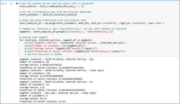
Interpretation: Customers on a month-to-month contract with DSL internet service are more likely to churn after an average of nearly 4 months. The segment has a modest proportion of senior citizens.

Business Impact: The churn in this segment may be related to dissatisfaction with the DSL service or the flexibility of a month-to-month contract.

Strategies:

Customized DSL Packages: For DSL users, especially in areas where Fiber optic might not be available, offering customized packages with relevant add-ons can enhance satisfaction.
Tech Support for DSL Users: Since DSL technology might face specific issues, specialized tech support can enhance user experience.

Improvement Recommendations: Offering incentives for longer-term contracts or improving DSL service quality could reduce churn. Tailoring packages for senior citizens may also engage this demographic more effectively.

Model Improvement: Consider features related to DSL service quality or customer feedback to predict churn more accurately in this segment.

2. Segment: Contract — Month-to-month, Internet Service — Fiber optic

A more modern and faster option, Fiber optic internet could be influencing customer satisfaction positively or negatively. Are customers churning because of higher costs or staying because of better performance?

Interpretation: This segment has a significant number of customers using fiber-optic services with a month-to-month contract. They tend to stay longer (average tenure around 19 months), and there is a substantial proportion of senior citizens.

Business Impact: This segment might be churning due to price sensitivity, especially among senior citizens who might find fiber-optic services expensive.

Strategies:

Bundling with Fiber Optic: For customers using Fiber optic, bundling high-speed internet with premium streaming services or advanced security features might add value.
Onboarding Support for Fiber Optic Users: Helping new Fiber optic users understand and utilize the full potential of their service can increase satisfaction and retention.

Improvement Recommendations: Offering special discounts for senior citizens or bundles that combine fiber-optic with other services might increase retention.

Model Improvement: Incorporating features related to pricing and customer feedback on fiber-optic services could enhance predictions.

3. Segment: Contract — Month-to-month, Internet Service — No

Interpretation: Customers without internet service and on a month-to-month contract churn quickly (average tenure of 1 month), with no senior citizens in this group.

Business Impact: This segment might represent a low-engagement or low-value customer base that is not interested in internet services.

Strategies:

Special Offers for No Internet Users: Understanding why certain customers opt not to use internet service and offering specialized packages or incentives might convert them into internet users.
Community Engagement: Creating community forums or support groups for users to share experiences, ask questions, and receive support can foster a sense of belonging.

Improvement Recommendations: Understanding the needs of this segment and offering tailored non-internet packages might increase retention.

Model Improvement: Focus on non-internet related features and consider different clustering or segmentation techniques to understand this group better.

4. Segment: Contract — One year, Internet Service — Fiber optic

Interpretation: Customers with a one-year contract and fiber-optic internet service have a high average tenure (around 56 months) and a moderate proportion of senior citizens.

Business Impact: This segment likely represents a more stable and committed customer base that is satisfied with the fiber-optic service.

Improvement Recommendations: Continue to engage this segment with loyalty programs and ensure consistent quality in fiber-optic service.

Model Improvement: Analyzing feedback and usage patterns within this segment can provide more granular insights into customer behavior and help in fine-tuning the predictions.

Analyzing Geographical Trends:

Churn might also be influenced by the geographical location of customers. Regional preferences, availability of services, local competition, and market conditions can all play a role.

Strategies:

Regional Marketing Campaigns: Targeting marketing efforts based on regional preferences and needs can increase effectiveness.
Expanding Service Availability: Analyzing areas with high churn due to lack of service options and expanding availability can capture lost market share.
Local Partnerships: Collaborating with local businesses to offer bundled services or discounts can create a community-centric brand image.

Continuous Monitoring and Improvement:

Churn analysis is not a one-time effort. Continuous monitoring and iterative improvements are key to staying ahead of customer needs and market trends.

Strategies:

Real-Time Churn Prediction: Implementing real-time churn prediction algorithms can provide early warnings about potential churn, allowing proactive engagement.
Customer Feedback Loops: Regularly collecting and analyzing customer feedback can lead to continuous improvements tailored to the evolving needs of each segment.
Competitor Analysis: Staying aware of competitors’ offerings within each internet service segment ensures that the service provider remains competitive and aligned with market expectations.

Overall Recommendations:

Customer-Centric Approach: Tailoring offerings based on customer segments and needs can improve retention.
Focus on Service Quality: Ensuring consistent quality across different internet services can reduce churn.
Leverage Contract Types: Encourage longer-term contracts with incentives or bundles.
Enhance Model with More Features: Including more features related to customer feedback, service quality, pricing, and personalized interactions can make the churn prediction model more robust and actionable.

These insights can guide business strategies and model enhancements to address customer churn more effectively across different segments. These customer-centric approaches not only enhance satisfaction and retention but also foster a brand image that is responsive, innovative, and in tune with customer needs. By embracing a data-driven, agile approach to customer engagement, service providers can transform the challenge of churn into an opportunity for growth and differentiation.

Conclusion:

The article Part1 and Part2 have presented a thorough exploration of customer churn prediction, delving into both the exploratory data analysis (EDA) and predictive modeling stages using XGBoost. This tutorial offers a valuable guide for anyone interested in the practical application of machine learning to real-world business problems. The tutorial has demonstrated a systematic approach to understanding, analyzing, and predicting customer churn, providing key insights into customer behavior, trends, and patterns.

While the focus has been on customer churn prediction, similar methodologies could be applied to other business challenges such as credit risk assessment and prediction of loan defaults. The principles of Exploratory Data Analysis (EDA), predictive modelling, and business interpretation are transferable across various domains. For instance, the Random Forest algorithm can be a robust choice in predicting loan defaults, with its ensemble of decision trees working together to enhance predictive accuracy. In the area of credit risk assessment, a Support Vector Machine (SVM) can provide clear classification boundaries, managing both linear and non-linear data patterns. Moreover, for more complex insights and predictions, Neural Networks might be a better model choice. These models exemplify the adaptable and extensive capabilities of machine learning in addressing diverse business challenges.

As emphasized at the beginning of the article, a professional data analyst’s role goes beyond mere number-crunching. Transforming raw data into actionable business wisdom is a valuable asset that guides informed decisions and innovative strategies. The case study of customer churn prediction epitomizes this transformation, where data-driven insights inform strategies to enhance customer loyalty and reduce revenue loss.

I have compiled all the code into code snippets for your reference.

#Step 5: Feature Engine  

# Feature Scaling
      from sklearn.preprocessing import MinMaxScaler
      
      scaler = MinMaxScaler(feature_range=(0, 1))
      scaled_features_df = scaler.fit_transform(data_df[["tenure", "MonthlyCharges", "TotalCharges"]])
      scaled_features_df[0]

# Feature Extraction
      data_df2 = data_df.copy()
      
      data_df['customerID'].head(2)
      
      data_df['customerID-part1'] = data_df['customerID'].apply(lambda x: x.split('-')[0])
      data_df['customerID-part2'] = data_df['customerID'].apply(lambda x: x.split('-')[1])
      
      data_df = data_df.drop(['customerID', 'customerID-part1', 'customerID-part2'], axis=1)

# Feature Building
        data_df['InternetService'].value_counts()
        
        data_df['InternetSpeed'] = data_df['InternetService'].apply(lambda x: 0 if x == 'No' else 10 if x == 'DSL' else 150)

# Feature Selection
        threshold = 0.99
        for rowIndex, row in corrmat.iterrows(): #iterate over rows
            for columnIndex, value in row.items():
                if rowIndex != columnIndex and value > threshold:
                    print(f"{rowIndex}  -  {columnIndex}  -  {value}")

# Encoding Categorical Feature
        encoded_data_df = encode_categorical_features(data_df)

        cols_to_drop = ['OnlineSecurity_No internet service', 'OnlineBackup_No internet service', 
                        'DeviceProtection_No internet service', 
                        'TechSupport_No internet service', 'StreamingTV_No internet service', 'StreamingMovies_No internet service']
        encoded_data_df = encoded_data_df.drop(cols_to_drop, axis=1)

        encoded_data_df.shape

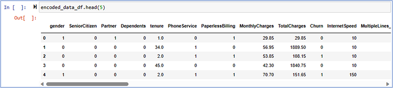
        encoded_data_df.head(5)

#Step 6: Model Training
 
# Data split
        from sklearn.model_selection import train_test_split
        
        #separating our input data from the labels
        encoded_data_df_Y = encoded_data_df['Churn'].copy()
        encoded_data_df_X = encoded_data_df.drop('Churn', axis=1)
        
        #we do a first 80/20 split between training set and the rest (= val + test) AND we shuffle
        train_x, rest_x, train_y, rest_y = train_test_split(encoded_data_df_X, encoded_data_df_Y, train_size=0.8, shuffle=True)
        
        #we split the previous 20% of the dataset in half to get test and validation, no need to shuffle again
        val_x, test_x, val_y, test_y,  = train_test_split(rest_x, rest_y, test_size=0.5, shuffle=False)


        print(f'train x/y - {train_x.shape} / {train_y.shape}')
        print(f'val x/y - {val_x.shape} / {val_y.shape}')
        print(f'test x/y - {test_x.shape} / {test_y.shape}')

# XGBoost and Decision Trees

        !pip install xgboost


        import xgboost as xgb
        
        #count(negative instances) / count(positive instances)
        scale_pos_weight = encoded_data_df['Churn'].value_counts()[0]/encoded_data_df['Churn'].value_counts()[1]
        
        #used for evaluation of the trees/estimators
        eval_set = [(val_x, val_y)]
        
        #configure the xgb classifier object
        xgbClassifier = xgb.XGBClassifier(objective="binary:logistic", 
                                          random_state=33, 
                                          n_estimators=50, 
                                          max_depth=4, 
                                          learning_rate=0.3, 
                                          min_child_weight=2, 
                                          scale_pos_weight=scale_pos_weight,
                                          eval_metric='aucpr')
        
        # "fit" the model on the data = launch the training process.
        fit_model = xgbClassifier.fit(train_x, train_y, eval_set=eval_set, verbose=True, early_stopping_rounds=10)


        pred_train_y = xgbClassifier.predict(train_x)
        
        pred_test_y = xgbClassifier.predict(test_x)

#Step 7: Model Evaluation

        xgb.plot_importance(fit_model,max_num_features=20)
        plt.show()

    #### Visual representation of your trees

        !pip install graphviz
        
        print(f'Number of sub trees: {len(fit_model.get_booster().get_dump())}')
        print(f'best sub decision tree: {fit_model.best_iteration}')
        
        from xgboost import plot_tree
        #plot_tree(fit_model, num_trees=1, rankdir='LR')
        xgb.to_graphviz(fit_model, num_trees=fit_model.best_iteration, rankdir='LR')

#1. Confusion Matrix
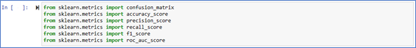
        from sklearn.metrics import confusion_matrix
        from sklearn.metrics import accuracy_score
        from sklearn.metrics import precision_score
        from sklearn.metrics import recall_score
        from sklearn.metrics import f1_score
        from sklearn.metrics import roc_auc_score
        
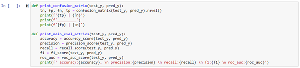
        def print_confusion_matrix(test_y, pred_y):
            tn, fp, fn, tp = confusion_matrix(test_y, pred_y).ravel()
            print(f'{tp} | {fn}')
            print(f'_________')
            print(f'{fp} | {tn}')
            
        def print_main_eval_metrics(test_y, pred_y):
            accuracy = accuracy_score(test_y, pred_y)
            precision = precision_score(test_y, pred_y)
            recall = recall_score(test_y, pred_y)
            f1 = f1_score(test_y, pred_y)
            roc_auc = roc_auc_score(test_y, pred_y)
            print(f' accuracy:{accuracy}, \n precision:{precision} \n recall:{recall} \n f1:{f1} \n roc_auc:{roc_auc}')
        
        print_confusion_matrix(test_y, pred_test_y)
        
        print_main_eval_metrics(test_y, pred_test_y)
        
      
#2. KFold cross validation

        from sklearn.model_selection import cross_val_score, cross_val_predict
        from sklearn.metrics import SCORERS

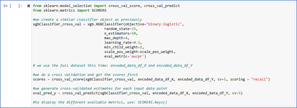
        #we create a similar classifier object as previously
        xgbClassifier_cross_val = xgb.XGBClassifier(objective="binary:logistic", 
                                          random_state=33, 
                                          n_estimators=50, 
                                          max_depth=4, 
                                          learning_rate=0.3, 
                                          min_child_weight=2, 
                                          scale_pos_weight=scale_pos_weight,
                                          eval_metric='aucpr')
        
        # we use the full dataset this time: encoded_data_df_X and encoded_data_df_Y
        
        #we do a cross validation and get the scores first
        scores = cross_val_score(xgbClassifier_cross_val, encoded_data_df_X, encoded_data_df_Y, cv=5, scoring = "recall")
        
        #we generate cross-validated estimates for each input data point 
        xval_pred_y = cross_val_predict(xgbClassifier_cross_val, encoded_data_df_X, encoded_data_df_Y, cv=5)
        
        #to display the different available metrics, use: SCORERS.keys()
        
        print(f'recall across all iterations: {scores}')
        
        
        print_confusion_matrix(encoded_data_df_Y, xval_pred_y)
        
        
        print_main_eval_metrics(encoded_data_df_Y, xval_pred_y)

#3. Overfitting and Underfitting

        xgbClassifier_overfit = xgb.XGBClassifier(objective="binary:logistic", random_state=33, 
                                                  max_depth=20, reg_lambda=0, n_estimators=400)
        overfit_model = xgbClassifier_overfit.fit(train_x, train_y, eval_metric="aucpr")
        
        
        print(f'Number of sub trees: {len(overfit_model.get_booster().get_dump())}')
        
        over_pred_test_y = xgbClassifier_overfit.predict(test_x)
        over_pred_train_y = xgbClassifier_overfit.predict(train_x)
        
        
        print_main_eval_metrics(train_y, over_pred_train_y)
        
        
        print_main_eval_metrics(test_y, over_pred_test_y)
        
#4. Hyperparameter Tuning

        from sklearn.model_selection import RandomizedSearchCV, GridSearchCV
        
        params = {'max_depth': np.linspace(3,7, 8, dtype=int),
                  'n_estimators':np.linspace(45,55, 5, dtype=int),
                 'reg_lambda':np.linspace(0.75, 1.5, 10, dtype=float),
                 'min_child_weight':np.linspace(1.5, 3, 10, dtype=float),
                 'learning_rate':np.linspace(0.1, 0.4, 10, dtype=float)}
        
        eval_set = [(val_x, val_y)]
        
        xgbClassifier_HPO = xgb.XGBClassifier(objective="binary:logistic", 
                                          random_state=33, 
                                          scale_pos_weight=scale_pos_weight,
                                          eval_metric='aucpr')
        
        search = RandomizedSearchCV(xgbClassifier_HPO, param_distributions=params, random_state=33, n_iter=50,  
                                    cv=5, verbose=1, n_jobs=4, return_train_score=True)
        
        search.fit(train_x, train_y, eval_set=eval_set, early_stopping_rounds=10)


        print(f"best_params:{search.best_params_}")
        print(f"best_score:{search.best_score_}")

        pred_HPO_test_y = search.best_estimator_.predict(test_x)

        print_main_eval_metrics(test_y, pred_HPO_test_y)

#Step 8: Customer Churn Prediction

        number_of_churn_predictions = sum(pred_HPO_test_y)
        print(f"Number of customers predicted to churn: {number_of_churn_predictions}")
        
        
        
        # Get the indices of the test set where churn is predicted
        churn_indices = test_x.index[pred_HPO_test_y == 1]
        
        # Get the corresponding rows from the original DataFrame
        churn_customers = data_df2.loc[churn_indices]
        
        # Merge the churn predictions with the original data
        churn_analysis_df = pd.merge(churn_customers, data_df2, left_on='customerID', right_on='customerID', how='inner')
        
        # Segment by 'Contract_x' and 'InternetService_x' (or any other feature of interest)
        segments = churn_analysis_df.groupby(['Contract_x', 'InternetService_y'])
        
        # Analyze each segment
        for (contract, internet_service), segment_df in segments:
            print(f"Segment: Contract - {contract}, Internet Service - {internet_service}")
            print(f"Number of customers: {len(segment_df)}")
            print(f"Average tenure: {segment_df['tenure_x'].mean()}")
            print(f"Proportion of Senior Citizens: {segment_df['SeniorCitizen_x'].mean()}")
            # Add more analyses as needed

If you found this article helpful, I’d appreciate it if you could show some love with a few claps at the bottom of the page. Don’t hesitate to leave your insights or feedback in the comments, and feel free to pass this along to your friends and follow me on Medium.

Some other articles from Jing Chen

Want to connect ?

Follow me on Medium
Connect me on LinkedIn