
A Complete Introduction To Time Series Analysis (with R):: The ACF and PACF functions
In the last article, we discussed the stationarity, causality, and invertibility properties of ARMA(p,q) process, along with the conditions required to ensure these, and how to verify them. In this article, we will see how these properties, in particular, stationarity and causality greatly simplify our task of finding the ACVF, ACF, and PACF.
ARMA(p,q) as a Linear Process
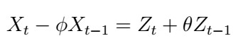
Recall from this article that a linear process is no more than a stationary time series which has the representation
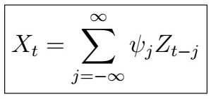
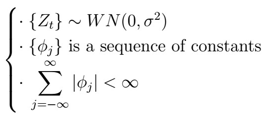
satisfying
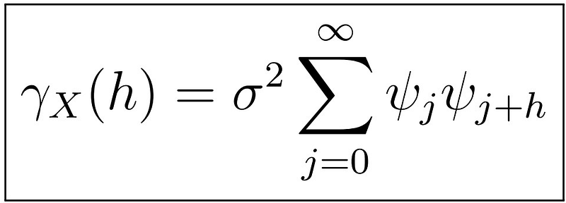
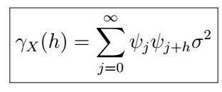
Further, we saw in this article that when the underlying random variables of such a process where white noise, then the autocovariance of such process can be written as
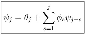
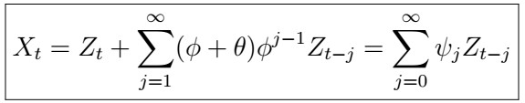
Now, from the previous article, we saw that if our ARMA(p,q) process is causal, we can find coefficients phi such that
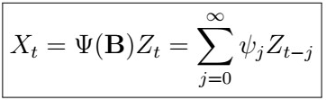
which is indeed a linear process with coefficients
Note that we can see the Psi polynomial as a “ratio” of the Theta and Phi polynomials,
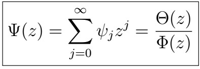
Thus, we can simply use the psi coefficients to find the ACV!
Worked Example
Let’s take a look at a fully-worked example with the ARMA(1,1); assume we have such a process given by
Now, we could use the recursive formula to find a casual representation. Such representation has the form
where
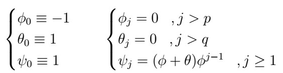
.Then, using the formula
we find
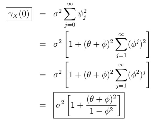
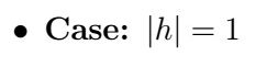
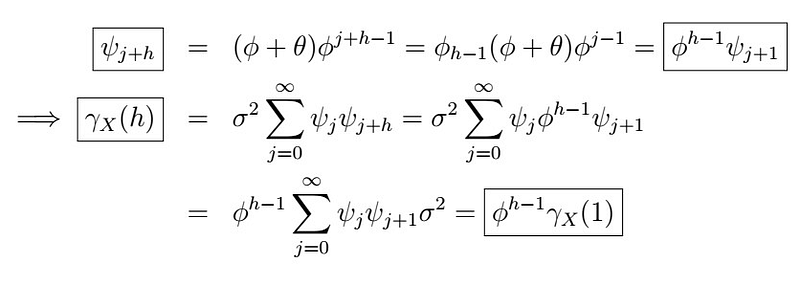
and that’s it! Needless to mention, once we know these forms, finding the ACF is trivial. Finding such nice, closed forms can get a bit messy with the infinite summations and the algebra, but otherwise, it is a pretty straightforward process. Thankfully, unless you are learning this material for academic purposes or pure enjoyment, most of the time you won’t find yourself calculating this by hand. In later articles, we will fully immerse ourselves in thorough examples in R, so you can see how everything connects. For now, let’s end this article with a review of the PACF :).
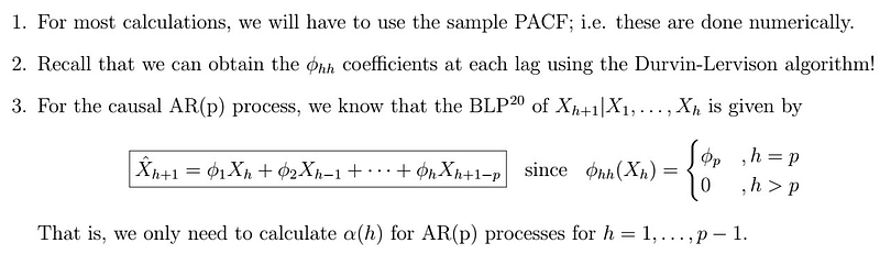
The PACF
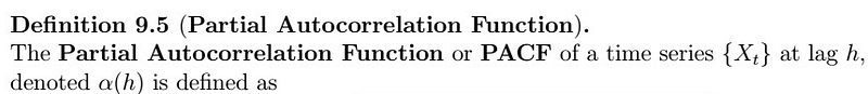
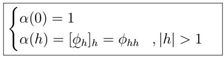
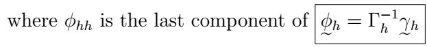
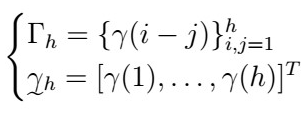
Of course, the sample PACF uses the sample autocovariance equivalents.
Remark
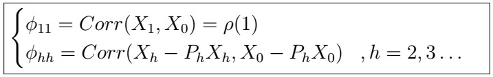
What is the PACF measuring?
The PACF measures the association of X_{h+1} and X_{1}, adjusting for X_{h}, X_{h-1}, … , X_{2}. That is, it tells us how much correlation is due to the furthest lag X_{1} with the actual observation we are looking at, having adjusted for the association of all other intermediate lags. More explicitly,
Check out some examples using the PACF in R here, but we will revisit it soon with ARMA processes :).
How to R
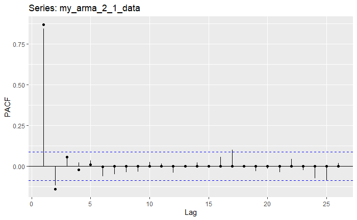
Let’s take a look at a quick example by simulating an ARMA(2,1) process, and inspecting how its ACF and PACF behave. As in the last article, we start by specifying its coefficients into an appropriate format:
Next, we make use of the arima.sim function to simulate our given ARMA(2,1) process:
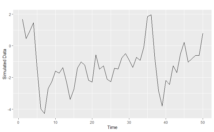
We can also plot the resulting process:
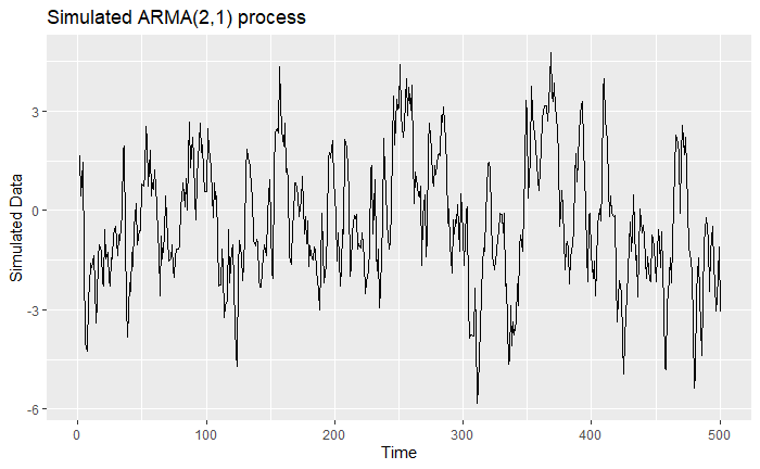
Note how hard it is to take a look at a Time Series plot and figure out whether it is stationary! If we take a look at the data, it looks like we “don’t” have a trend, and you could even think that there are seasonal components, the variability kind of changes from time, etc. We can also loop into a small window of the process:
There seems to be some autocorrelation here, but it is still very hard to tell precisely what it is. Instead, let’s take a look at the ACF and PACF:
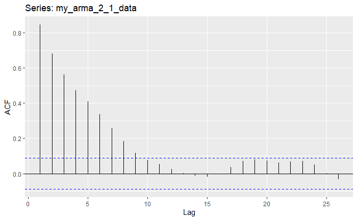
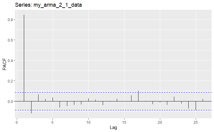
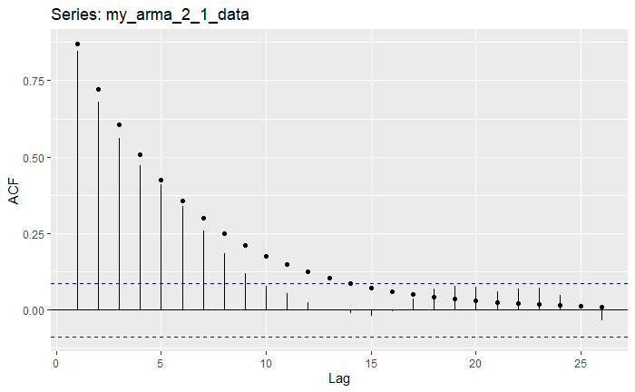
Here, one important thing to see is that even though in the ACF there are a number of lags that go outbounds, the PACF shows us that when adjusting for the correlation in between, this becomes significantly smaller. We can use the true ARMA(2,1) coefficients that we specified above to compute the theoretical ACF and PACF quantities and compare them to the sample ones as follows:
We can observe that these values closely correspond to the ones in the plots:
Next time
And that’s it for now! In the following articles, we will take a look at forecasting with ARMA(p,q) processes, along with some cool examples in R. Stay tuned, and happy learning!


