
A Complete Introduction To Time Series Analysis (with R):: Linear processes II
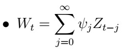
Last time, we left off at the representing Linear Processes in terms of the backward-shift operator:
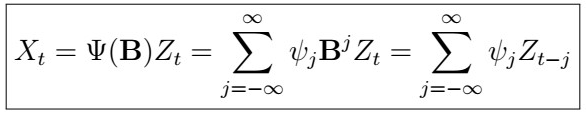
where Psi is the polynomial such that
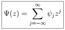
, and we said that this representation will be useful later, especially when dealing with ARMA, ARIMA, and SARIMA models. This time, we will continue exploring some important properties and concepts related to Linear processes. Let’s start by giving a simple but illustrative example!
MA(p)
As you may have guessed from the MA(1) process, the MA(p) is just a generalization to going p-steps back into time, collecting past noise as a weighted average. Indeed, we can write
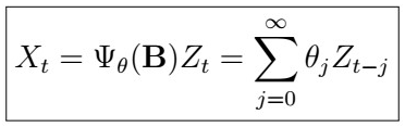
that is, we have that
. Not so hard eh! We will see more examples of linear processes later.
More Cauchy-Schwarts
Well, here we go again. Guess why the following proposition is true?
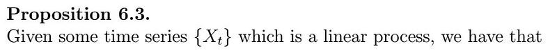
Don’t worry too much at understanding why this is the case, but for the curious: both the expectation operator and the absolute value can be seen as norms from the L1 and probability inner product spaces respectively, so that we can apply Cauchy-Schwarts over and over. If none of this made any sense, don’t worry about it. If you would like, however, to get an idea of what I’m talking about, check my linear algebra review and probability review appendices, in which I have collected a bunch of these concepts, theorems, and definitions.
Wold Representation Theorem

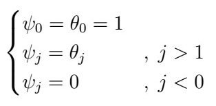
where

is an infinite moving average of noise terms, satisfying
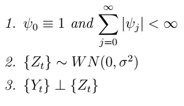
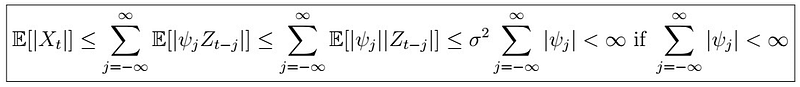
So what is the Wold Representation Theorem saying? If we have any stationary series, then we can split it into a linear process and an infinite moving average, where both of these contain different terms. Why is this important? A consequence is that every second-order weakly-stationary process is either a linear process or can be transformed into one by substracting a deterministic component!
Autocovariance function of Linear Processes
Now, how is all of this useful? Remember the definition of the autocovariance function for a stationary series:
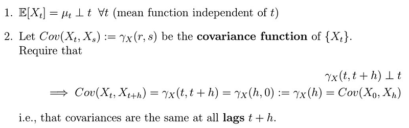
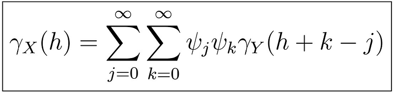
It turns out that given the nature of linear processes, we can generalize the form of its autocovariance function! So any process that is a linear process will have one form for its ACVF. Pretty convenient! Right?

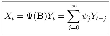

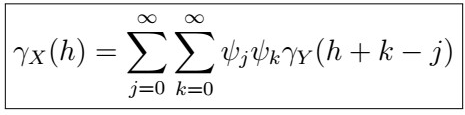
where
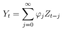
Let’s understand what this is saying: the third equation says that Y_{t} is a linear process. Then, we have that X_{t}, which is composed of a weighted sum of Y_{t}’s is also a linear process, and further, we know the form of its ACVF. How do we know this? We can just derive it from the definition!
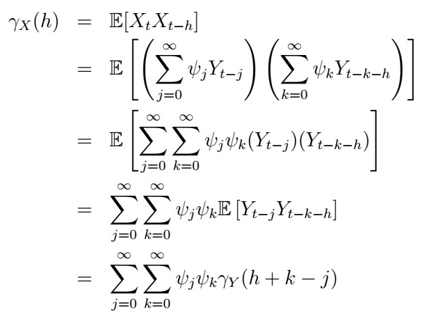
Which follows just by simple re-ordering, and the fact that we can interchange expectation and summation since our series are summable by definition.
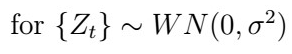
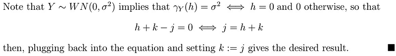
Now, how about if Y_{t} is also white noise? That makes things much easier! In such a case, we have that
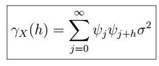
So that if we know what the psi coefficients are, all we have to do is to plug them in and we are done! Now, why is this the case?
Example
Let’s now see how we can use this in an example.
Getting the ACVF of the AR(1) process
Suppose that X_{t} is an AR(1) process, that is
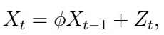
where the X_{t} and the Z_{t} are independent at any time point. Then X_{t} is a linear process, and cane be written as
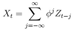
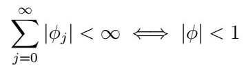
where
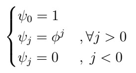
satisfying
Since {Z_{t}} is a stationary process (White Noise is stationary!), then X_{t} is also stationary, and we can easily find its ACVF using the formula from before!
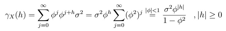
and you can verify that this is the same formula as we derived at the beginning of the series , in the AR(1) section.
Next time
That’s it for today! Next time, we will take a brief look at the operators we have seen so far, as it will step aside from a bit and take a look at some important operators we have seen so far, along with an example of how useful they will be.


