
A Complete Introduction To Time Series Analysis (with R):: Stationary processes
In the last article, we discussed two important models with structure: the trend decomposition model and seasonal variation. We said that one of the most important steps in the general strategy for time series analysis was to remove the signal, i.e., remove either the estimated trend or seasonality or both. In this section, we will talk about stationary processes, and what it means to be stationary. Let’s dive right into it!
Stationary Processes
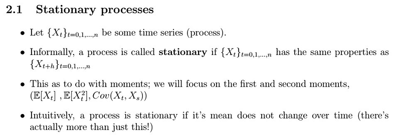
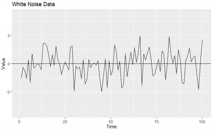
Let’s consider some time-series process Xt. Informally, it is said to be stationary if, after certain lags, it roughly behaves the same. For example, in the graph at the beginning of the article, we see that although there is some fluctuation, the points seem to wander around zero, in particular, this is called a mean-zero process. We will define more precisely what this means next. For this purpose, we will focus on studying the second moments, i.e., mean, covariance, and variance of a certain process.
There are two kinds of stationarity: weak stationarity and strong stationarity. Both of these are defined below. If you need a refresher on expectation, covariance, variance, and distributions, make sure to check these notes from Standford’s CS229 machine learning course.
Let’s now check these definitions.
Weak stationarity
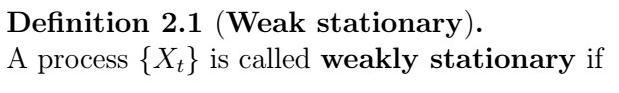
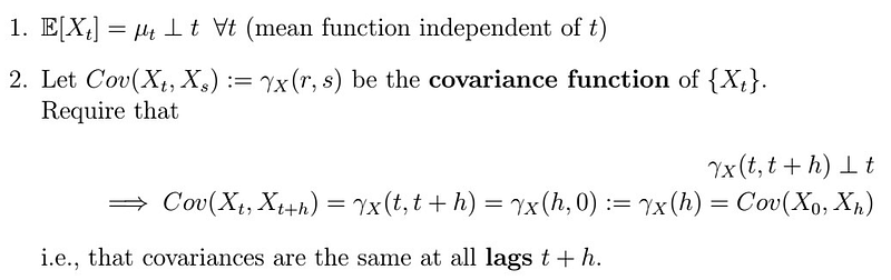
The first point says that we have some mean, whatever it might be, which is a function independent of t, that is, it does not depend on any particular timestep. In the second point, we define the autocovariance function by the letter gamma, of two observations at times t and s. In order for the process to be stationary, we require that the covariance function of Xt at lags t and t+h is also independent of t. That is, we only have covariances for lags 0,1,…,m, say, after which, it should get repeated again.

Strong stationarity
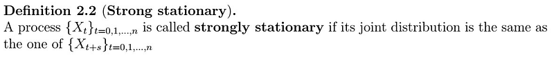
This time, we require in addition that the joint distribution of the process shifted by a lag s is the same. This is indeed much stronger than the previous definition.
Ok, so what do we do with this? It turns out that we would much more like to work with stationary series than non-stationary ones, and in fact, most of the theorems and propositions that we will are based on these assumptions. If a series is not stationary, the idea is to make it into one (we will see how in a later article ).
Autocorrelation function
The autocovariance function might seem a little funky at first, but it is in fact, along the autocorrelation function (ACF), is an essential tool for Time Series analysis. Let’s recall the definition of the correlation between two random variables:
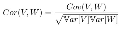
This tells us how strongly related or “similar” are two variables. The ACF of a time series uses the exact same concept, except that using the autocovariance formula we saw before; that is
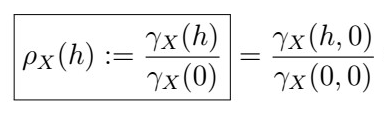
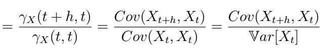
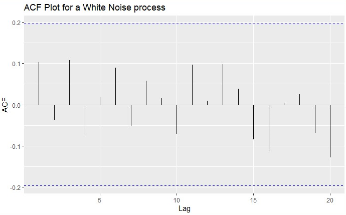
So we see that this is no more than the good old correlation. As you should know, this ranges between -1 (indicating negative correlation) and 1 (indicating positive correlation). The main idea is that, if we plot the ACF, a stationary series will show most or all of the points within certain confidence bounds, without any predictable pattern, like in the following plot:
Next time
Next time, we will see illustrate these concepts with various processes that are and are not stationary, along with the How to R sections to produce these plots. Stay tuned!


