
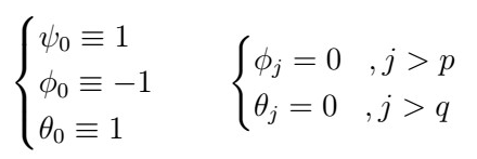
A Complete Introduction To Time Series Analysis (with R):: ARMA processes (Part II)

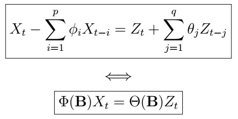
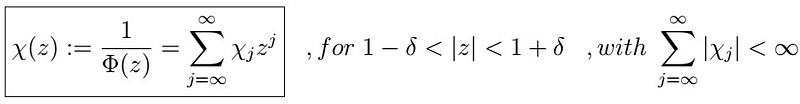
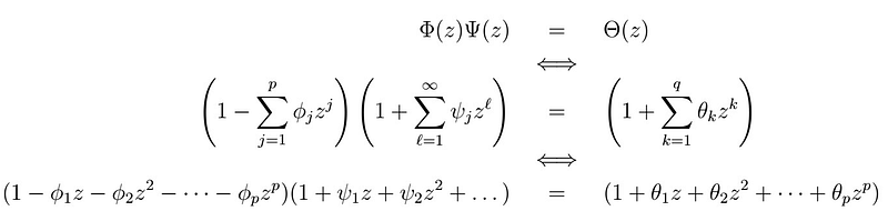
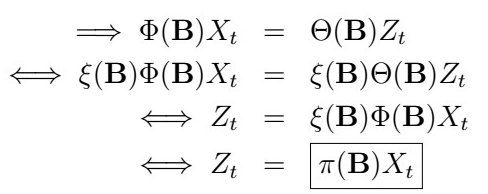
In the last article, we saw that a general ARMA(p,q) process can be written, with the help of the autoregressive and moving-average operators as
. We also discussed three important properties of an ARMA process:
- Stationarity
- Causality (current observation-only depends on the past)
- Invertibility (can correctly represent current noise as a function of the observations from the past)
We illustrated this with the ARMA(1,1) process, and we saw that we had to put some restrictions in order to ensure that the properties above are satisfied. This time, we will generalize these ideas to the ARMA(p,q). For this, we will make use of the basics of complex numbers, so if you need a review on the essentials, you can take a look at this article.
The Unit Disk
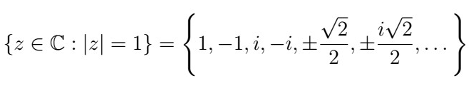
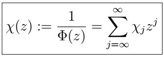
Let’s first recall the unit disk defined on complex numbers, given by the set
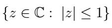
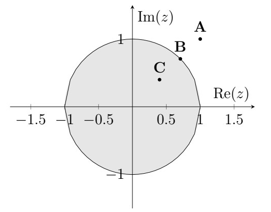
,that is, the set of all complex numbers with modulo less or equal to 1. Graphically, this is
The unit circle is the same set, but holding with strict equality
Now, recall the ARMA(1,1) process, given by

From the previous article, it follows that in order to ensure stationarity, we need
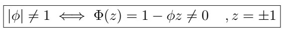
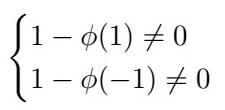
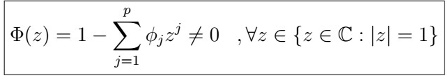
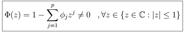
How can we generalize this to the ARMA(p,q)? In simple terms, we would like to have no roots of the autoregressive Phi polynomial on the boundary of the unit circle, that is, no roots on
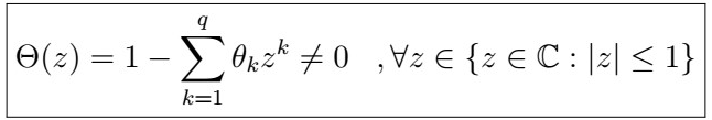
Before morving forward, we will need the following proposition:
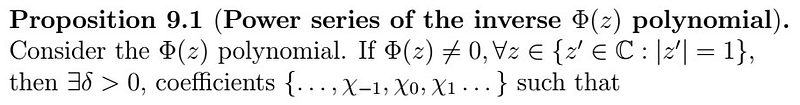
In simple words, this proposition is saying that if the Phi polynomial is not zero, then for all complex numbers in the unit circle, we can find coefficients with an arbitrarily close distance such that the power series of the inverse Phi polynomial is convergent. The proof of this relies on analysis, so we won’t go into that here. Armed with this, we are now ready to give formal definitions/characterizations of stationarity and causality in ARMA(p,q) processes.
Roots in the unit disk
We generally visualize the inverse roots as they are easier to visualize inside the unit circle than outside. We will use the following graph as reference.
Stationarity of ARMA processes
A stationary solution to an ARMA(p,q) process {X_{t}} exists and is also unique iff
that is if there are no roots of the autoregressive Phi polynomial on the unit circle. In the unit disk graph, and assuming we are plotting the inverse roots, only point B would violate the condition.
Causality of ARMA processes

Equivalently, if there are no roots of the autoregressive polynomial Phi on or inside the unit circle, that is
If we plot the inverse roots on the complex plane like in the graph we presented before, points A and B would violate this condition. That is, we would like to have the inverse roots strictly inside the unit disk!
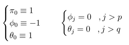
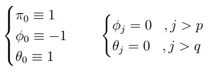
Finding the coefficients of a causal ARMA process
Now that we know how to determine whether an ARMA(p,q) process is causal, how can we find the corresponding coefficients of the causal representation?
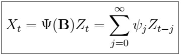
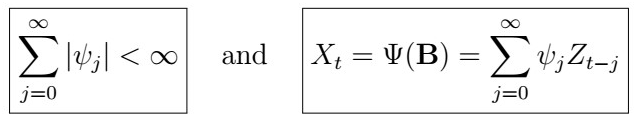
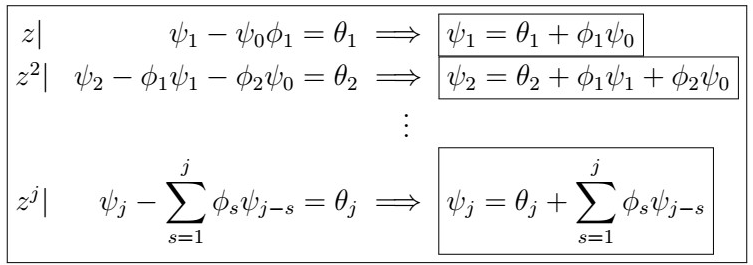
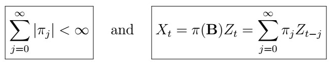
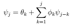
where the psi coefficients are determined by the recursive equation
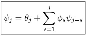
where
Proof
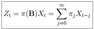
Recall that if {X_{t}} is causal, we have that
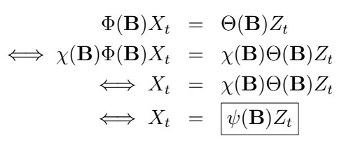
where
Note that this implies that
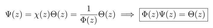
We can make use of this fact to recursively solve for coefficients of the Psi polynomial. Written more explicitly, we have
Note that
Then, we can simply start comparing coefficients on both sides of the equation yields
Invertibility of ARMA(p,q) processes

or equivalently, if the are no roots of the moving average Theta polynomial on or inside the unit circle, that is
Visually, we would like to have the inverse roots strictly inside the unit disk:
, so that in the graph above, only the inverse root A would violate invertibility conditions.
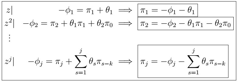
Finding the coefficients of an invertible ARMA process
Similar to before, we can also find corresponding coefficients whenever the process is invertible.
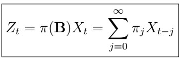
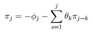
where the pi polynomial coefficients are determined by the recursive equation
satisfying
Proof
We can show this in a similar way as we did before. First, recall that if {X_{t}} is invertible, we have that
This implies that
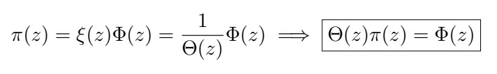
Once again, we can make use of this to obtain the pi coefficients, by noticing that
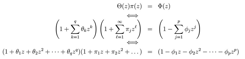
and
Then, comparing coefficients we obtain
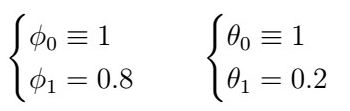
Concrete Example
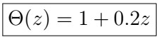
Let’s now see a concrete example using specific values for an ARMA(1,1) process. In particular, consider {X_{t}} ~ ARMA(1,1), given by
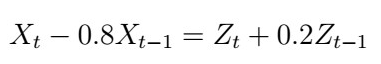
This implies that
We see that the corresponding AR(1) polynomial is
From which we see it has a zero at 1.25. Clearly, this falls outside the unit circle, which indicates that there exists an ARMA(1,1) process that is stationary and causal. Now, to find the causal representation of the process, we use the recursive formula
. Writing out the first couple of terms:
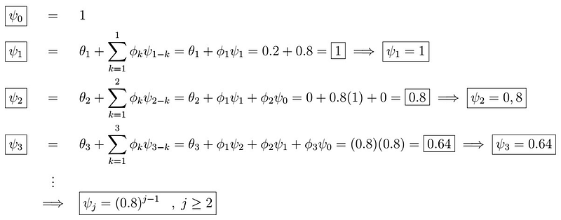
Which we can then, in turn, plug into
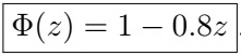
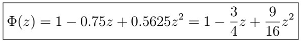
Similarly, the corresponding MA(1) polynomial is
which has a root at z=-5. This also falls outside the unit circle, which ensures that our process is invertible. Now, in order to find the inverse representation, we use the formula
, yielding
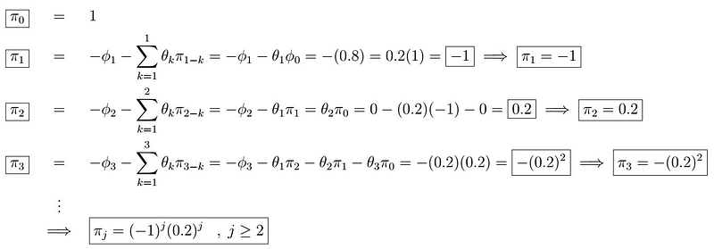
Which we can then plug into
One last brief example
Let’s consider the process X_{t} ~ ARMA(2,1) given by

Then, we have that
We can use the quadratic formula
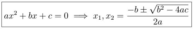
to find the roots, yielding
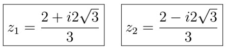
We can then calculate the modulus for each:
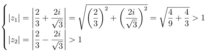
Therefore we have no roots inside the unit circle, ensuring that our process is stationary and causal. However, notice that for the AR(1) polynomial
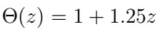
has a zero at -0.8, which indicates that the process is not invertible!
How to R
Now, we are going to simulate a couple of examples of plotting and examining polynomial roots for ARMA(p,q) processes in R. First, we import the required libraries:
Next, we are going to simulate an ARMA(2,1) process. . First, we simply create two vectors which will represent our models’ coefficients, various ARMA models:
Next, we can numerically obtain the roots of both the AR(2) and MA(1) corresponding polynomials using the polyroot function as follows:
Note that we prepend an extra 1 at the beginning for a valid polynomial. We can now visually inspect these roots using the forecast::plot.armaroots package as below:
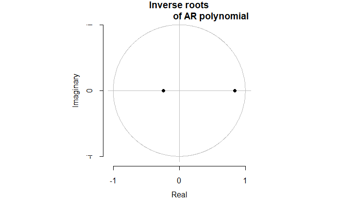
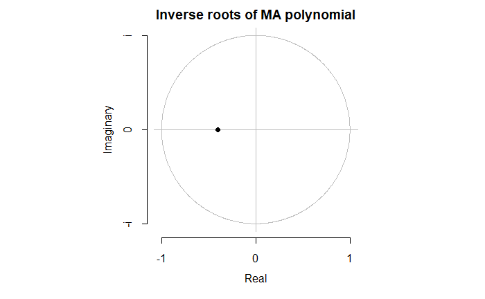
From these, using the conditions given before, we can see that since the inverse roots lie within the unit circle for both polynomials, we have a process that is stationary, causal, and invertible. If, for instance, one of our AR roots didn’t appear in the plot above inside the circle, then our process would no longer be causal or stationary.
Next time
That’s it for now! In the next article, we will take a look back at both the ACF and PACF, applied to ARMA(p,q) processes. Stay tuned, and see you next time!


