
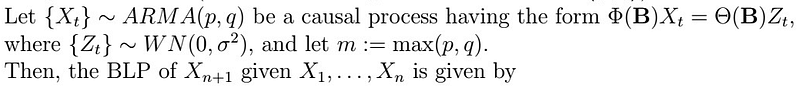
A Complete Introduction To Time Series Analysis (with R):: Prediction III: Forecasting with ARMA(p,q) models
We have come a long way from first exploring the idea of models with way too little or too much dependence, to the structured ARMA(p,q) models that aim to balance this by taking into account not only dependence between observations, but between their random noise at different timesteps. In the “Prediction II: Forecasting” section, we studied the best linear predictor along with two algorithms to help us find the BLP coefficients and make predictions: the Durbin-Levinson algorithm and the Innovations algorithm. In this article, we will see how to extend these ideas to produce predictions for ARMA(p,q) models. Before starting, I strongly suggest you review the first article on the Innovations algorithm since this one builds directly on that one. Let’s now get into it!
Innovations Algorithm for ARMA(p,q)
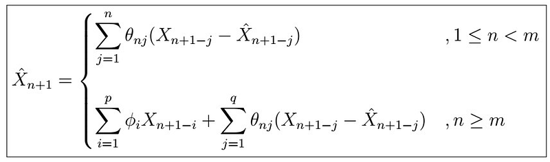
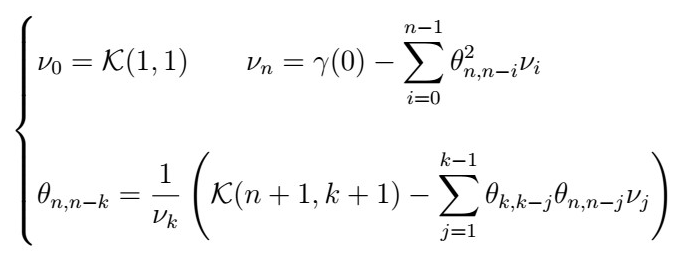
where the theta coefficients are determined by the recursive computations
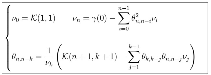
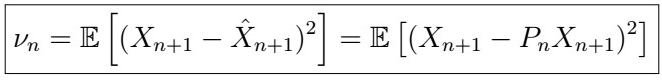
and nu satisfies
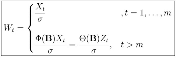
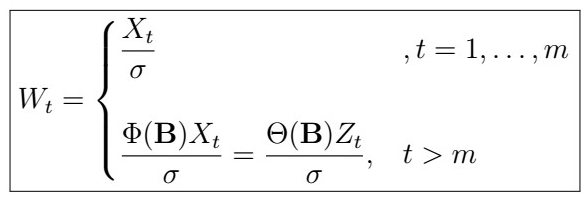
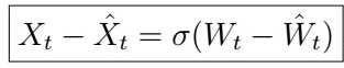
Further, let W_{t} be defined by

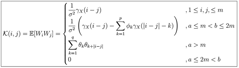
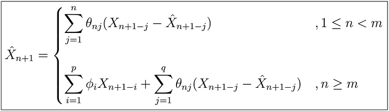
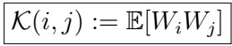
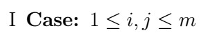
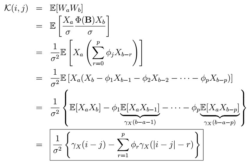
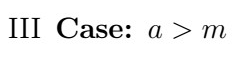
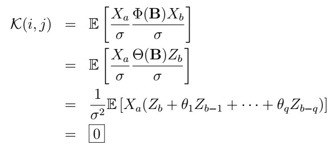
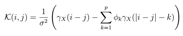
Before we proceed with the proof which actually provides insight into the formulation of the algorithm, let’s try to understand what it is saying. We first consider an ARMA(p,q) process and propose that the BLP of the observation X_{n+1} can be found by the formula above, dependent on some theta coefficients. These coefficients, in turn, also obey a set of recursive formulas, depending on the function K(i,j), reminiscent of the ACVF. Indeed, note that these depend on the random variables W_{t} rather than the original ones, these ones being a sort of normalized version of them. Let’s now see why that is the case, and how it is useful.
Proof
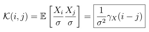
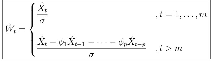
First, we will show the last equation presented. We define W_{t} as above, and see that for t > m this is well-defined, because

Now, assume that p,q ≥ 1 , and define
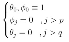
. However, allow theta and phi zero coefficients. Define

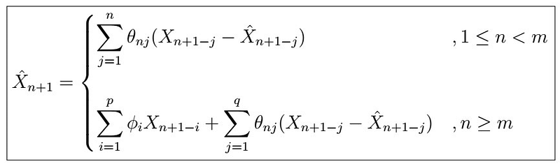
Now, we consider the W_{t} sequence and apply the version of the Innovations algorithm that we had previously studied to it. This gives
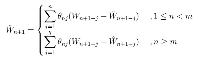
where for n ≥ m , the summation only goes up to q , since

Therefore, W_{t} is a linear combination of X_{t} iff X_{t} is a linear combination of W_{t}. Now, note that the BLP for Y|X_{1}, … , X_{n} is the same as the BLP for Y|W_{1}, … , W_{n} . Thus, we have that
Finally, since
as well, we can deduce that
. Notice that this formula is nothing more but the Innovations we had previously derived! We can therefore conclude that
The rest of the equations for computing the actual coefficients and nu_{n} come directly from the Innovations algorithm version we first discussed. You can compare this formula to the one we had before:
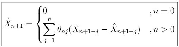
For which you can see it is almost the same, except that this one extends for the broader ARMA(p,q) model. Let’s conclude with an example :)
Example

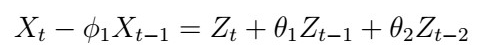
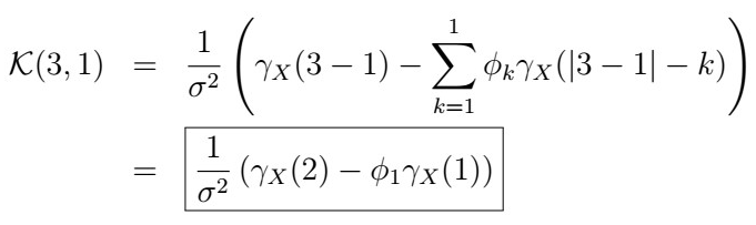
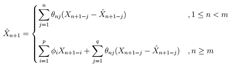
Given X_{1} and X_k{2}, what is the BLP of X_{3} using the innovations algorithm? First, recall the equations
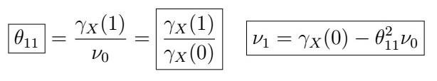
Here, we have that m=2, and we need to find the coefficients
n=1
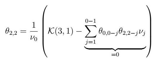
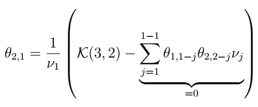
n=2
— k=0

, so we use
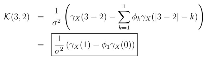
Plugging in,
— k=0

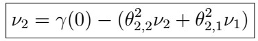
Now, to find v2 we use
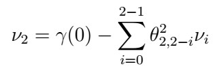
That is
Now we can recursively compute the predictions for X_{1}, X_{2}, X_{3} as follows:
n=0
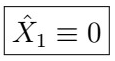
n=1
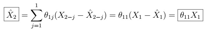
n=2
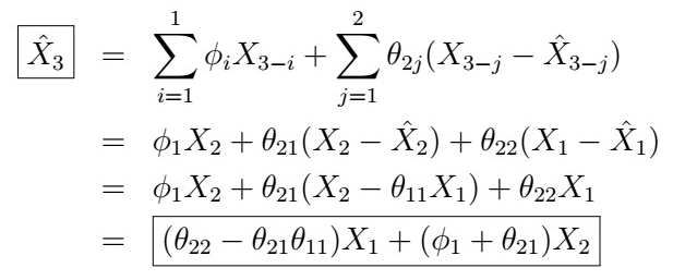
At this point, we can simply plug all the values for theta that we found before.
Next time
In the next article, we will start to embark on a number of algorithms to estimate the ARMA(p,q) coefficients, not a trivial task!


