
A Complete Introduction To Time Series Analysis (with R):: Best Linear Predictor (Part I)
In chapter 5 of this article series, we found that the best predictor of the n+h-th lag is given by the conditional expectation of X_{n+h} given X_{n}, that is
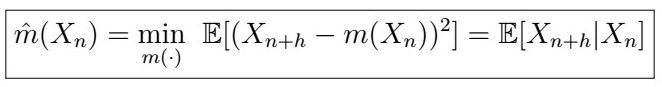
or extending to using all observations X_{1}, X_{2}, … , X_{n} , we can predict X_{n+h} by the conditional expectation of X_{n+h} given X_{1}, …, X_{n}. Further, we found that the actual form of this expectation when using only the last observation is given by
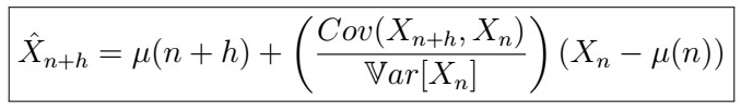
where, in the case that X_{n} were stationary this further simplified to
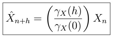
In this article, we will further explore a more precise and clear representation by using once more the principles of calculus optimization and linear algebra. Let’s jump into it!
The Projector Operator
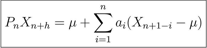
Note that that the formula for the stationary case for predicting X_{n+h} given X_{n} is a (rather boring) linear combination. We would like to extend this to the case in which we use all observations X_{1}, X_{2}, …, X_{n}, say by finding some coefficients a_{0}, a_{1}, …, a_{n}, that is
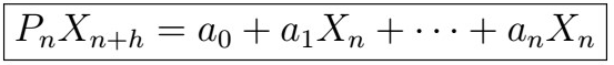
, where P_{n} is called the projection operator. But how can we find these coefficients? Just as we did before, we will attempt to minimize the MSE of P_{n}X_{n+h} (prediction) and X_{n+h} (actual).
Best Linear Predictor of X_{n+h} given X_{1}, X_{2}, … , X_{n}
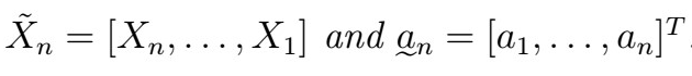
Let {X_{t}} be any stationary series. Let,
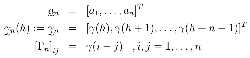
That is, we have
- A vector of n coefficients.
- The Gamma vector at lag h.
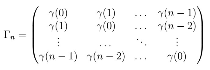
- The Gamma matrix, whose entries are given by
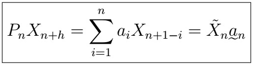
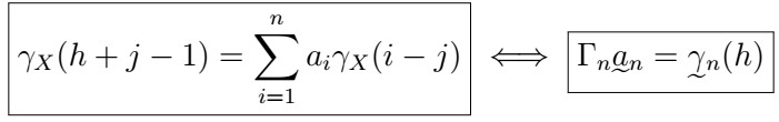
Then, the Best Linear Predictor of X_{n+h} given X_{1}, X_{2}, … , X_{n} is given by
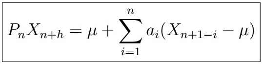
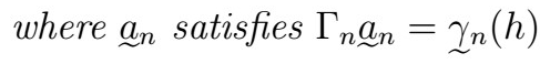
where the coefficients satisfy
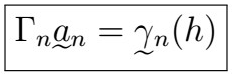
This is saying that we can predict the n+h-th lag by using all observations from 1 to n along with some coefficients given by solving the equation above. This is really useful as we can simply solve for the system above, and voilà! We now have a way to make systematic predictions by plugging estimates of the ACVF function whenever appropriate.
Proof
Let’s see why the above is true. We first consider the minimization problem:
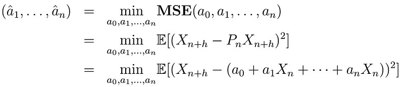
That is, we want to find coefficients that provide the smallest MSE. Note that the MSE is a convex function, which means that it is bounded below by zero. Therefore we can find at least one solution to
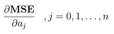
Under certain conditions satisfied by this optimization problem, we can interchange the expectation operator and the derivative, from which, after setting equal to zero, we obtain the equations
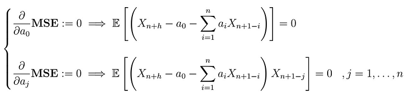
Solving the first one, we obtain
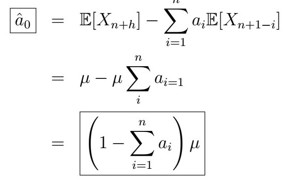
We can then plug this into the second equation(s), so that
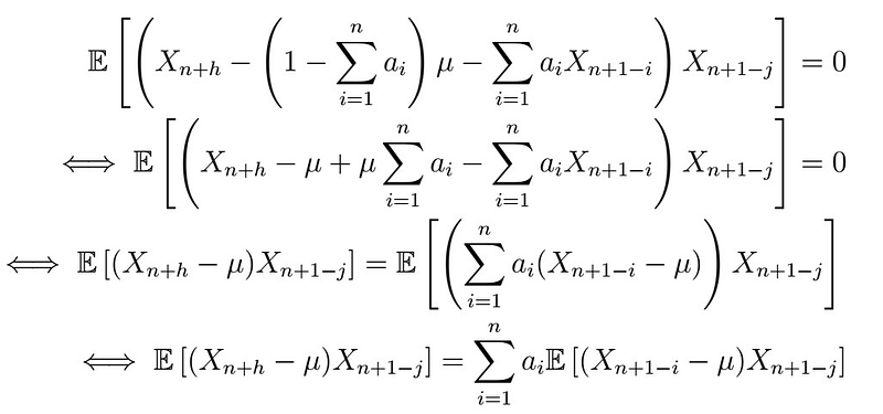
Note that in the second line, we simply expand the innermost parenthesis and that the expectation of any X_{i} is simply mu, as the series is assumed to be stationary. We then simply re-distribute the remaining terms. Now, remember that

, therefore the left side becomes

and similarly, with the expectation on the right side, we obtain

Plugging this back into what we had before, we have that
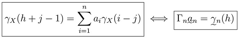
where
which follows as we simply can collect all the terms for all j, and then express the result it in vectorized form.
Remark
Note that this implies that
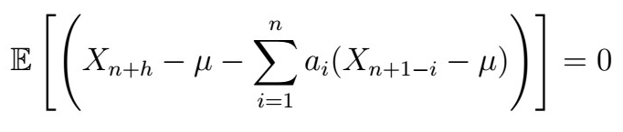
Further, if our time series process has mean zero, our predictor further simplifies to
where
MSE of the Best Linear Predictor
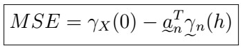
Remember that the MSE is also a way to measure the overall error of our predictor, which is why we would like to minimize it. As such, let’s see the actual form of it:
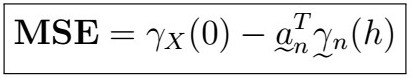
That is, the MSE is given by the variance of our time series at time 0, minus a linear combination of the weights and all the all the covariances from lag h to lag h+n-1 .
Proof
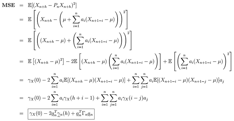
Let’s see what’s going on here:
- The first line is just the definition of the MSE.
- In the second line, we just plyg the definition of the projection operator.
- Third line, we arrange terms.
- In the fourth line, we expand the quadratic expression and distribute expectations.
- We see that the first expectation is simply the variance, or autocovariance at lag 0. For the second expression, we simply push terms not dependent on the index i inside the summation, and push the expectation operator inside per linearity property. The fourth term is simply the summation expansion of the quadratic term.
- The second-last comes as the expectations can be translated into autocovariances.
- Lastly, we vectorize the expressions using the gamma vector and matrix.
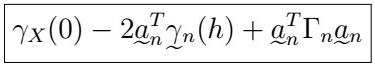
Let’s take a closer look at the last expression:
Now , recall that
, which we obtained from before, and note that
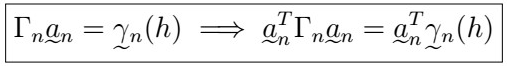
so we can simply replace the last term in the expression to obtain the result:
Remark
Note that if we have white noise, then
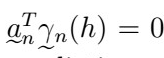
That is, we can’t explain anything! Otherwise, this expression gives us the MSE of our prediction.
Next time
And that’s it for today! It was a lot of math and calculations, but the important take-outs are the forms of the projection operators and the MSE. In the next article, we will see an example of how to apply this to a known time series, along with interesting things such as predicting a random variable in a time series from other random variables, and some important properties of the projection operator. Stay tuned, and happy learning!


