
A Complete Introduction To Time Series Analysis (with R):: Estimation of the ACF
Last time, we saw how to estimate the trend of any time series along with meaningful statistical properties such as unbiasedness and variance. This time, we will now proceed to build solid statistical estimates of the ACVF and ACF.
Asymptotic behaviour of the sample ACVF and sample ACF
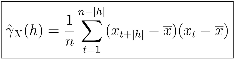
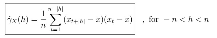
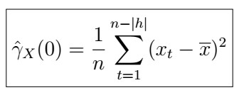
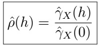
Recall the definition of the sample autocovariance function for any time series:
with
and further,
(If this seems confusing, recall that we defined these before in this article).
It turns out that these estimates are biased, but nonetheless consistent. That is, with little data, the expectation will not arrive at the actual true value but rather to a factor of it. However, since these are consistent, this tells us that the estimates will actually be better the more data we have.
- Note that in the summation, we only go up to n-|h| instead of n .
- However, we divide by n and also subtract the whole sample mean.
- It turns out this is also the best we can do when it comes to the estimation of the autocovariance! (proof out of scope).
Proof Sketch
The idea is first to solve that the sample ACVF is biased. Recall that for any random variable X

Therefore,
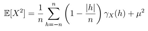
So all we have to do now is to calculate the expectation. Take your time processing what’s going on in the calculations:
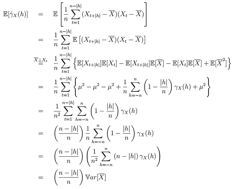
Let’s see what happened here:
- The first line is simply plugging in the definition.
- As the expectation is linear, we can put it inside the summation.
- By independence of the sample mean and every single observation (out of scope), We can expand the inner term and apply expectations independently.
- We translate these terms into mu and the second moment we found before, plug it in and cancel terms.
- In the fifth line, we have canceled terms and only the summation remains, so we just aggregate those.
- In the sixth line, note that no term depends on t, so we simply sum this factor and re-write again.
- We factorize one (1/n²) term from the inside of the summation and pull it just outside the sum.
- This is no more than the definition of the Variance of the sample mean estimator that we had found before! , times a factor.
So the bias is given by
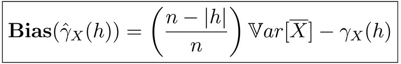
Note, however that as n goes to infinity, the bias goes to the variance of the sample mean minus the actual value.
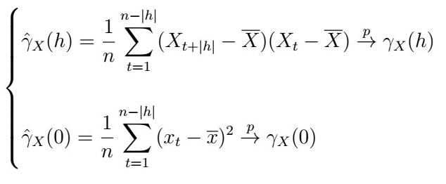
Now, if we want to show consistency, the idea is to use the L.L.N and Slutky’s Theorem to show that
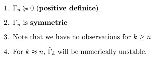
Aside: Gamma vector and Gamma matrix
So besides doing funky summations and statistics, what is the ultimate goal? The idea is that in order to perform inference about p(h), we need some distributional assumptions which make use of these estimators (for instance, building confidence intervals about the true values). We will first proceed to define two useful objects: the gamma vector and the gamma matrix.

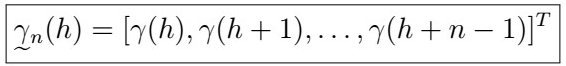
, and the sample version just uses the sample ACVF instead.

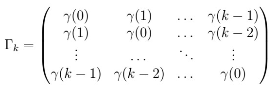
similarly, the sample version replaces its entries with the sample ACVF. In the rest of this article, we will only use the gamma vector, but both of this will be useful in future sections.
Properties
Joint distribution of sample (p(1), … ,p(k))
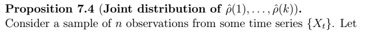
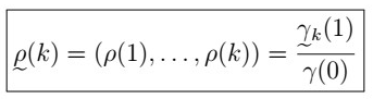
be the vector of all correlations up to k (note this is just the Gamma vector of 1 divided by gamma of 0), having some joint distribution F, say. Then, for large samples without large lags, we can approximate such distribution by
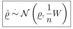
That is, the sample ACF vector follows a multivariate normal distribution with mean vector equal to the true ACF vector, and the variance above, where W is a covariance matrix with entries given by
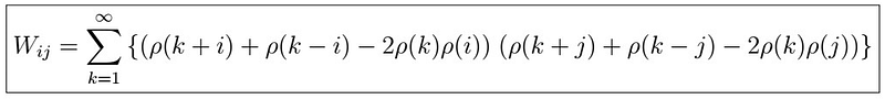
. This is a special case of Berlet’s formula. Not getting into the details of how this came about or how it is true, let’s see a couple of examples.
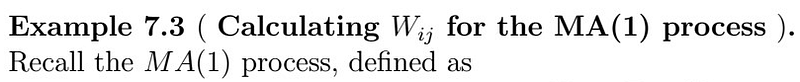
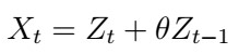

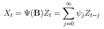
with coefficients
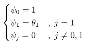
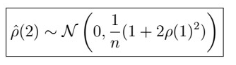
, and so it can be shown that
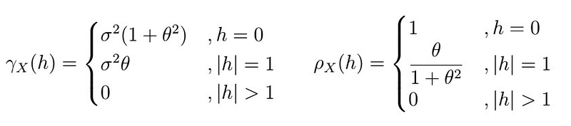
. In order to calculate
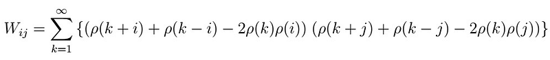
we first consider the case when i=j.
i=1
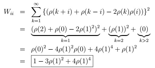
So that
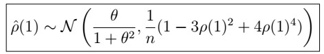
i>1
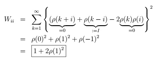
So that
Next time
That’s it for now! Next time, we will actually move back to forecasting by further defining the shape of the best linear predictor of a future observation given our data. Stay tuned, and see you next time!
Last time
Introduction to Time Series Operators


