
A Complete Introduction To Time Series Analysis (with R):: Introduction to Time Series Operators
In the last article, we explored some useful properties of linear processes, including the Wold’s Representation Theorem, as well as a very useful characterization of the autocovariance function of any linear process. In this article, we will roll back a little, and get a grasp of the different operators we have seen so far and giving a short illustration of how useful these can be when dealing with messy calculations involving time series. If you forgot some of these, you can take a look at the differencing article where I originally introduced some of these. Let’s jump to it!
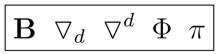
Backward Shift Operator
Recall that in the differencing section, we introduced the backward shift operator as
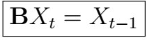
That is, this operator simply takes some observation at time t, and returns the previous one.
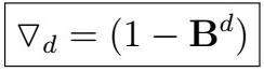
Difference Operator
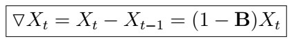
The difference operator is defined as
For instance, one application would look like the following:
And this can be done d times, as specified.
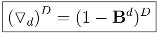
Lag-difference operator
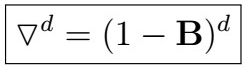
The lag-difference operator is defined as
Note the difference in the exponentiation! Although it is pretty clear, in the differencing section, we also saw an example showing that these lead to different algebraic results. In fact, notice that nothing restrict us from writing something like
Why would we ever do something like this? It turns out this will make sense much later in more advanced models such as the ARIMA and SARIMA models.
Big phi operator
A first definition of the Big phi operator is
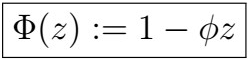
Does this remind you of something? If you were thinking the AR(1), props to you! Indeed, we have that

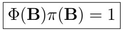
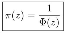
Pi operator
We define the Pi operator as
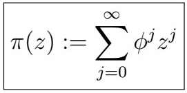
Why is the purpose of this operator? What if I told you that
How? We can simply apply the definitions and see that
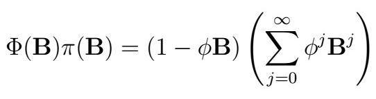
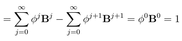
Like magic! This in fact implies that
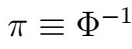
so it’s common practice to write
although this is not technically correct.
Example: Inverting the AR(1)
Armed with these operators, first notice that we can represent the AR(1) process as

Remember that the AR(1) is in fact, a linear process as well. We can easily show this using operators as follows:
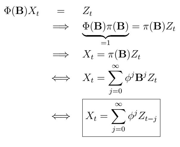
That was pretty convenient!
Next time
And this is it! With this, we close another major section. In the next articles, we will focus on the estimation of mean and variance parameters along with its statistical properties, which will in turn be useful for forecasting. Until next time!


