
A Complete Introduction To Time Series Analysis (with R):: Innovations Algorithm
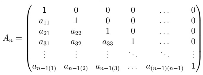
In the last article, we studied in depth the famous Durbin-Levinson algorithm, which allowed us to recursively compute the coefficients of the best linear predictor given by
satisfying the following
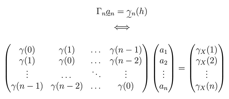
, without having to explictly invert the Gamma matrix. In this short article, we will take a look at the Innovations algorithm, another algorithm that will allow us to iteratively make predictions.
Innovations algorithm
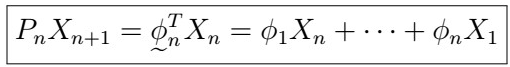
We will now take a look at the Innovations algorithm. First, we are going to re-define the BLP of X_{n} as follows:
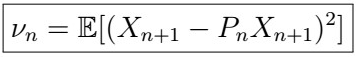
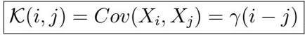
Next, we define the MSE as you might expect:
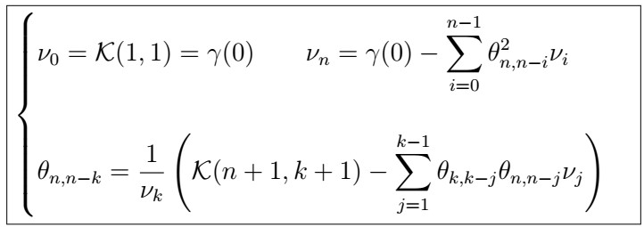
We define the one-step innovations as (prediction errors) as
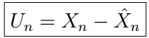
That is,
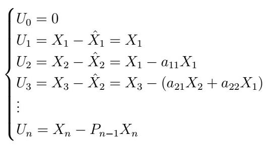
At this point, you can already see that each “innovation” is definininf the difference by adding one prediction at the time. In order to facilitate computations, we define the following vectors:
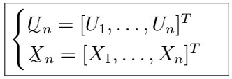
That is, this is just a collection of the observations and the innovations, defined as column vectors.

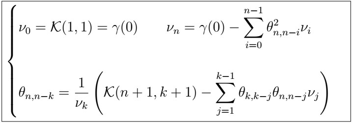
which contains a collection of coefficients for each BLP at each timestep. We now propose the next claim without proof:

This is why if we want to use this algorithm, we will actually want our series to be stationary, or to be turned into one, and be able to assess this using statistical tests and diagnostics. Now, provided that our A_{n} matrix is non-singular (therefore invertible), we can define the matrix
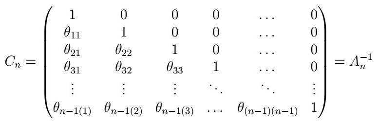
Now, we define the matrix
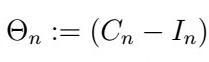
that is
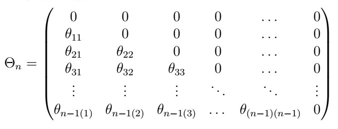
Which is the same matrix, without the diagonal 1’s. Then, we have, using some simply algebra that
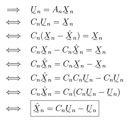
So that
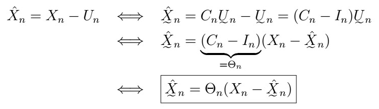
Now, why is this useful? Rememer that these are vectors, which means that we can use these step-predictions to make a new one as follows:
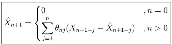
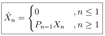
Finally, as you might expect, there is a way to compute thesre recursively. Let
Then, we can compute
and that’s it! The proof of correctness of this algorithm is rather involved, so I will not present it here, but if you are interested, you can check out these lecture slides. We will come back to this algorithm later when we show predictions for it.
How to R
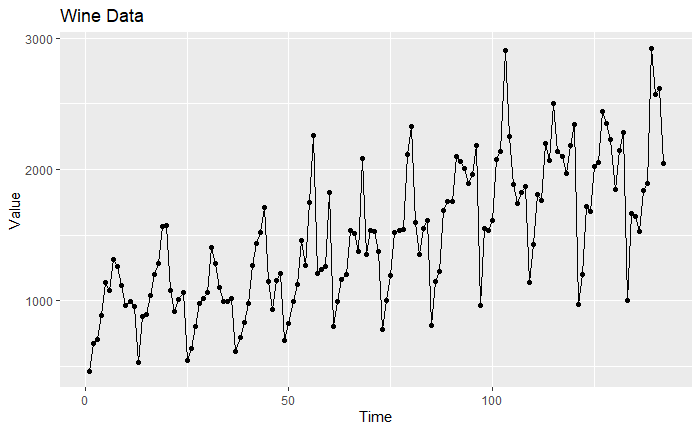
For this example, we will use wine dataset , already built-in in R. First, let’s import some libraries:
Next, let’s inspect the data. It looks as follows:
From documentation: “The wine dataset contains the results of a chemical analysis of wines grown in a specific area of Italy. Three types of wine are represented in the 178 samples, with the results of 13 chemical analyses recorded for each sample.” We will perform inference on this data using the Innovations algorithm in the itmsr package. Let’s now plot the data:
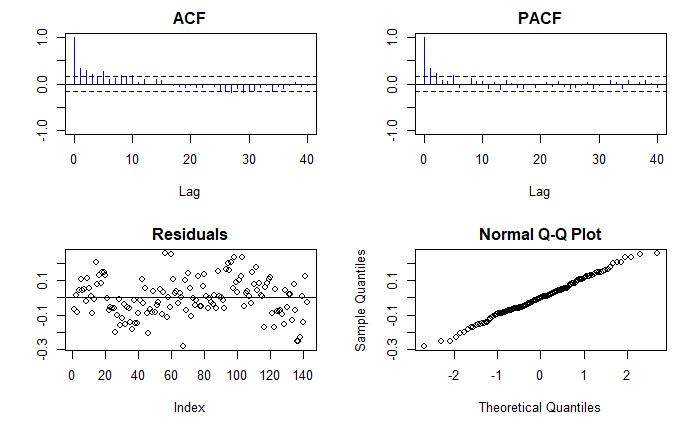
This data actually has a yearly seasonality, so we will use a lag of 12. We will fit a model implictly and then check for stationarity using the tests we presented before:
According to the tests, there is a strong evidence that the residual series is stationary. as we fail to reject the null hypothesis in the majority of the tests. We can also verify this visually with the diagnostic plots:
This is still not the best, but it is a good application of the Classical Decomposition model. We can also fit an ARMA(p,q) model as follows (we will study these next!). We can use these residuals to apply an ARMA(p,q) model on top:
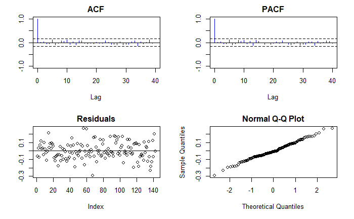
and we see that this one definitely looks stationary from the tests and diagnostic plots. Finally, we can use the calssical decomposition transformations and the fitted ARMA model to obtain predictions as follows:
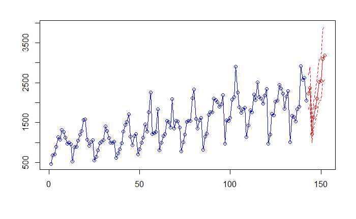
Which under the hood, uses precisely the Innovations algorithm.
Next time
This concludes the end of this chapter! In the next article, we will begin our discussion of ARMA processes, which will allow us to combine the power of AR(p) and MA(q) processes into one. Stay tuned, and happy learning!


