
A Complete Introduction To Time Series Analysis (with R):: Exogenous models
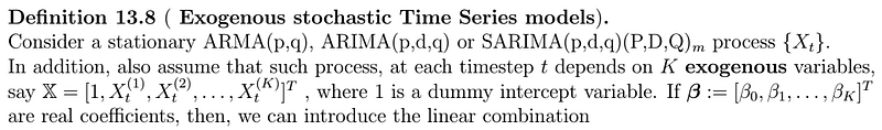
We have come pretty far into our analysis of univariate time series. So far, we have considered some sort of time-based stochastic process X_{t}, dependent on current and previous noise and itself. However, what happens when in addition, we would like to model our endogenous process as also being dependent on external factors, or exogenous variables? First, recall that the classical decomposition model states that
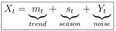
, whereX_{}
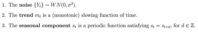
In exogenous models, we would like to include a number of external variables that will, in addition, contribute to the response. How can we do that?
Suppose that in addition to the response or target process X_{t}, we also had dependence at each timestep on an external variable, say X^(1)_{t}. Then, we could state such dependence in terms of the classical decomposition model as follows:
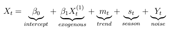
In this equation, we can clearly see the dependence of the random variable X_{t} on the exogenous variable, which interacts with the other components in an additive way. You can think of it as introducing the classical linear regression setting, except that now the random error includes the additional complexity of a time series process. In order to optimize such a model, we could use a variety of algorithms such as least squares or gradient descent. Although this approach, stated in the way above could work, we would like to extend this idea to K exogenous variables, and also to the ARMA, ARIMA, and SARIMA models we have previously studied. Let’s see how we can formally do this.
Exogenous Stochastic Time Series Models

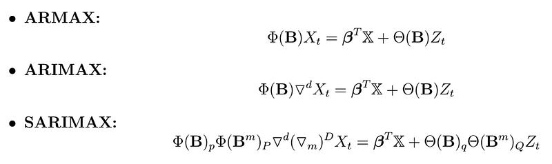
, where all the operators are described in the previous article. These models are also called Regression with ARMA/ARIMA/SARIMA errors.
Remark
Usually, optimization of all the previous models is done by maximum likelihood estimation using numerical methods such as quasi-Newton “hill-climbing” algorithms. Other methods include fast Bayesian methods, such as Hamiltonian Monte Carlo No-U-Turn Sampler (NUTS) development by Hoffman and Gelman (see https://arxiv.org/pdf/1111.4246.pdf), all out of the scope of this article. Model selection can also be done using the AIC, AICc, and BIC metrics, as described in previous articles.
Example

Such process can be written as
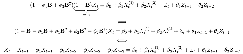
, where the process Y_{t} is an ARMA(2,2) after differencing (ignoring the regressors). We can solve the above expression for X_{t} to yield the following representation:
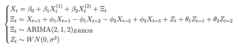
, where
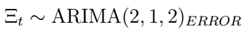
indicates that this model is a regression with ARIMA(2,1,2) errors. The coefficients
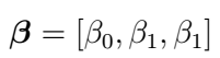
can then be found using regression on the expression for X_{t}. Note that if the process is stationary, it should follow that
How to R
Now we get to the fun part. As usual, let’s start by importing a couple of required libraries:
The following example is partially adapted from Forecasting Principles and Practice — 2nd Edition. We will be using the uschange data, which reports percentage changes in quarterly personal consumption expenditure, personal disposable income, production, savings, and the unemployment rate for the US, 1960 to 2016 (see this page). Let’s inspect the data at hand:
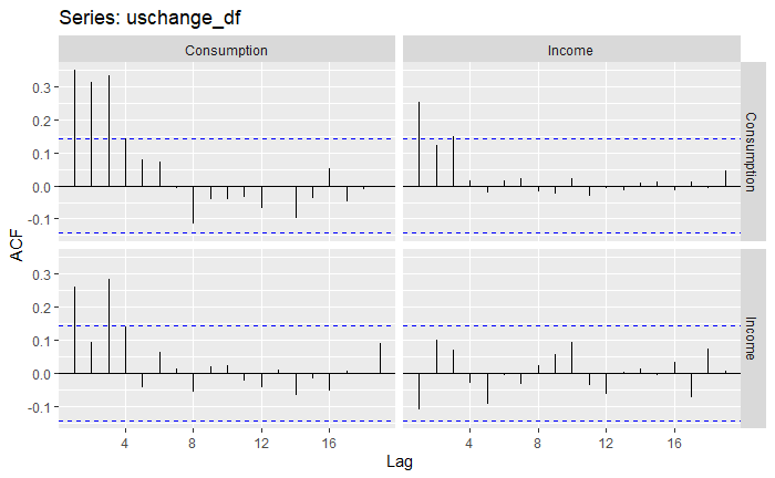
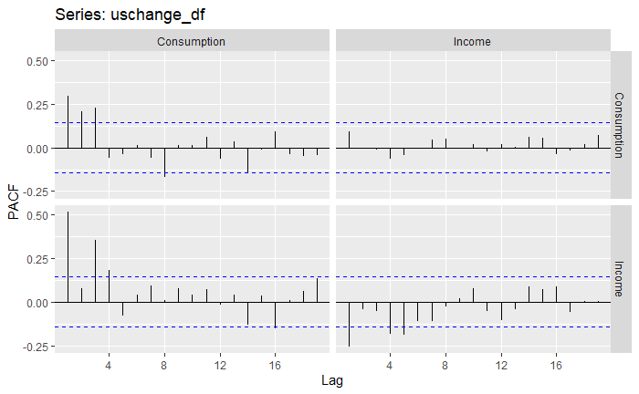
So far, we can see that we have data from 1970 to 2016, that the data is quarterly data (i.e. there is seasonality), and also that we have a variety of different columns. In this case, we will have as an assumption that “Income” has a direct impact on “Consumption”, our target variable. That is, we will use “Income” as an exogenous variable to the model. That being said, feel free to include more regressors later, and see how this affects performance! Let’s now plot the series jointly, as well as their ACF and PACF functions. The off-diagonal graphs, in this case, depict the covariance between both variables through time at different lags, but as we already assume that “Income” will have an impact on “Consumption”, we are mainly interested in the diagonal ones.
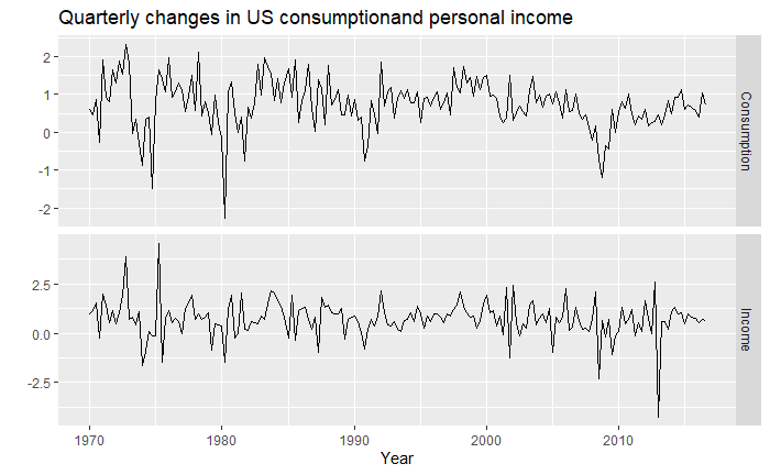
At first look, we can see that the “Income” exogenous variable is a lot more stationary already.
Classical Decomposition
Let’s take a closer look at the classical decomposition model for these two variables independently
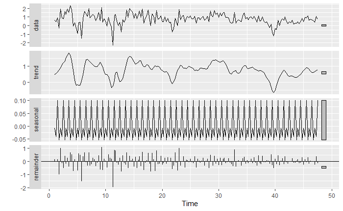
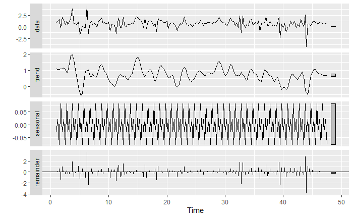
We can see that the “Income” exogenous variable is indeed a lot more stationary than the target random process. We can also see that there is indeed a seasonality pattern that could be captured. We will try both the ARIMAX and SARIMAX models to see which one provides a better fit.
Fitting and ARIMAX model
In order to fit an ARIMAX model, we will use the xreg argument when calling the auto.arima function. Note that now we are dealing with several variables, so that if the fitted model requires differencing, the R function Arima, implicitly used in auto.arima, will apply such differencing to all the variables before actually fitting the model.
It looks like our best model is the regression with AR(3) errors, or ARMAX(3,0) with the “Income” exogenous variable. In equations, this would look like the following:

In order to make the regression model more explicit, we can also write the model above as follows:
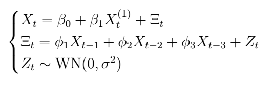
This representation makes it clear that the model is simply treated as a linear regression model, but in this case, the errors are modeled according to an ARMA(3,0) process.
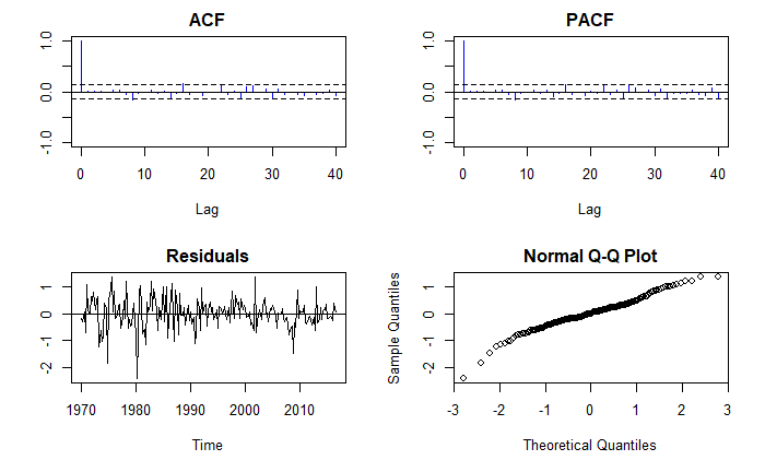
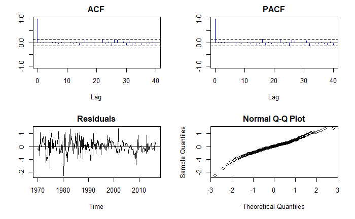
We can inspect these error ARMA process as we would do with any other:
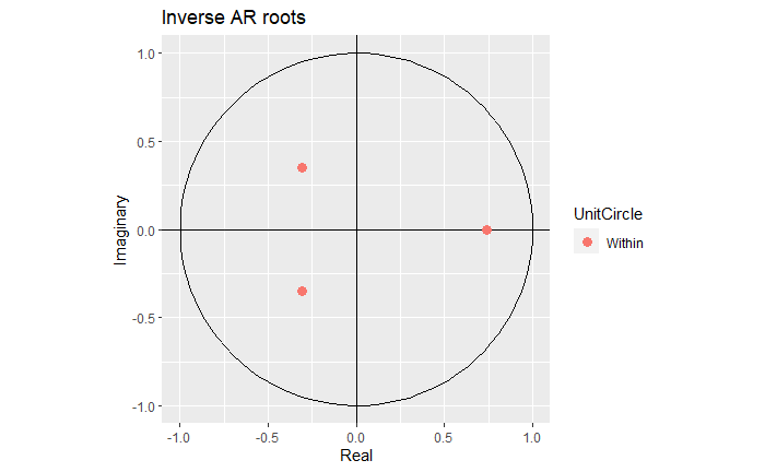
This indicates we have a causal, stationary process.
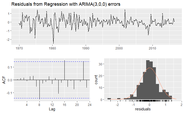
The residuals also seem more or less stationary although not entirely normal. Could a SARIMAX model do better?
Fitting a SARIMAX model
We will do the exact same, except that we will now allow the seasonal argument to be TRUE.
The model obtained is a regression model with SARIMA(3,0,0)(2,0,0)[4] errors. This can be written as

Although it is a bit cumbersome, you can see that such a model can be expressed in the regression form as before, where the error is then modeled as a SARIMA process as specified above (give it a try)! Let’s evaluate this model by inspecting the residuals:
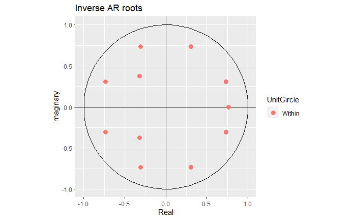
Note that in this case, we have 3X4=12 roots, coming from the non-seasonal AR(3) and seasonal AR(2) polynomials.
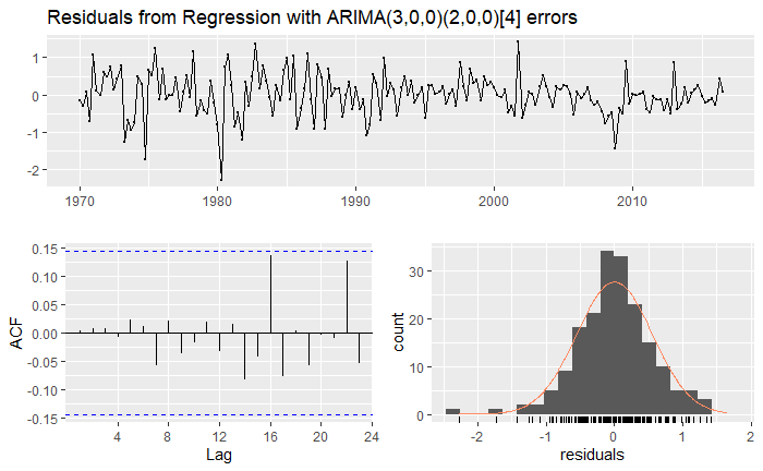
It would seem that this model isn’t much better. In such a case, we would opt to go with the first, simpler ARIMAX model, since it is easier to interpret.
Forecasting
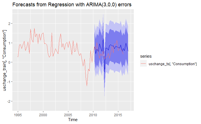
Of course, one of the most fun parts is making predictions with our model. The following code illustrates how to do this in R. Note that we re-train the model, but this time we perform a train-test split, only train on the train set, and predict on the testing one! This is because we want to asses the usefulness of our model on unseen data.
We see that even though our model does not perfectly match the actual data, it is actually not too far off from it, as even the 95% confidence intervals trap the actual data. We can also produce forecasts using the mean of the predictors, to obtain a more general but certain picture:
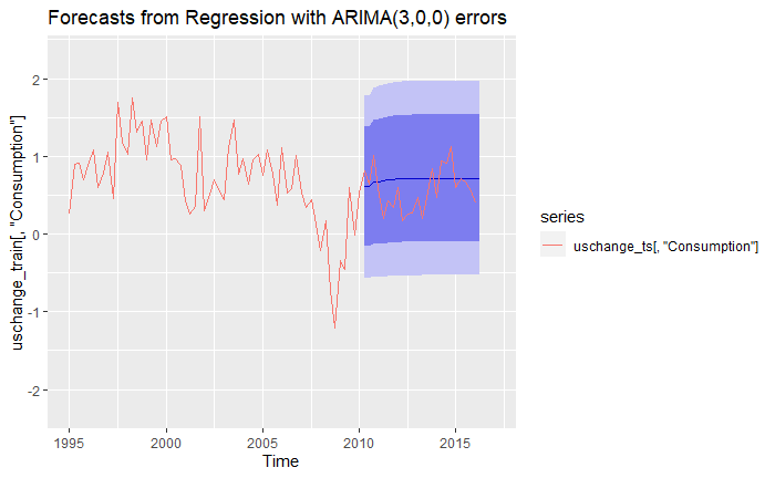
And behold the power of stochastic Time Series analysis with integrated exogenous variables!
Last words
And sadly, that concludes this series, “A Complete Introduction to Time Series Analysis”. Congratulations on having made it here!! It has been a rather long, but fun journey, and it almost makes me sad to end it all of a sudden here. Of course, the analysis of time series is much, much broader, and there is still a bunch of more advanced topics to cover, including vector autoregression models such as VAR, VARMA, and VARMAX for multivariate time series, as well as time series using deep learning techniques such as deep feed-word neural networks, CNNs, RNNs and LSTMs, and much more. In the future, I plan to perhaps initiate another series on these advanced techniques, or even expand to other languages such as Python, and/or expand these series as well. For the time being, I am really, really thankful to all my readers; thank you for your support, which really encourages me to keep writing articles weekly. This wouldn’t have been possible without all of you!! I will keep working hard to produce quality articles on python, statistics, data science, and machine learning every week or two.
In the meantime, feel free to head over a very fun example about using Time Series analysis on the stock market! (not saying that should!!! always follow professional advice, and trade at your own risk).


