
A Complete Introduction To Time Series Analysis (with R):: SARIMA models
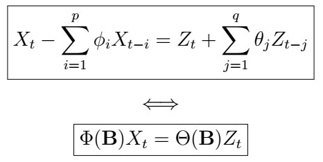
In the last article, we saw one important useful extension to the ARMA models: the Autoregressive Integrated Moving Average or ARIMA models, which formalize and integrate the differencing factor into the model. This time, we will see yet another very useful extension: seasonal component with the SARIMA models. But before we jump into the main topic, let’s recall the equation formulation of the ARMA(p,q) models in summation and operator forms.
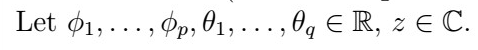
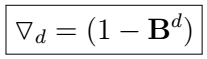
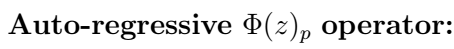
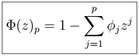
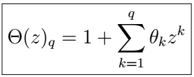
Autoregressive and Moving Average Operators
ARMA(p,q) processes
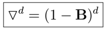
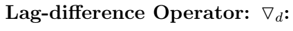
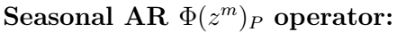
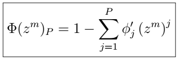
SARIMA Operators

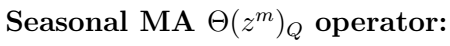
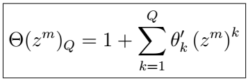
Seasonal Autoregressive Integrated Moving Average : The SARIMA(p,d,q)(P,D,Q)m process.


Written explicitly, this is

This process is often also called multiplicative seasonal ARIMA.
Example
Consider the SARIMA(1,1,1)(1,1,1)[12] process. Such process can be written in as

Here, we can interpret this process as having an ARIMA(1,2,1) component, implying that differencing twice will yield an ARMA(1,1) process, as well as a seasonal ARIMA(1,2,1) component with a period of 12. For instance, a (rather complicated) process that is based on monthly data might have such a configuration.
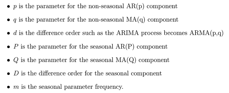
Model Selection
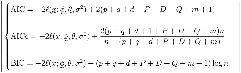
We will not go in-depth into the workings and more subtle properties of the SARIMA model, but you can see the similarities of the metrics above with the way they are used for ARMA and ARIMA models as we saw before. That is, we would perform model selection on the same dataset by choosing one or two of these criteria, and choosing the model with the lowest metric score.
Let us now get into a more practical example with R!
How to R
As usual, we start by importing a couple of libraries:
We will work on the elecequip data , which can be found in R datasets. THis data constists of the manufacture of electrical equipment: computer, electronic and optical products. Let’s have a glance at the data:
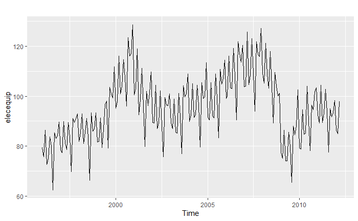
An interesting thing that we can notice here immediately is the period. We can take a good guess that there is a certain pattern that happens every year; indeed, we can use the stl function to estimate the seasonal component of the data, which we can in turn substract an inspect as follows:
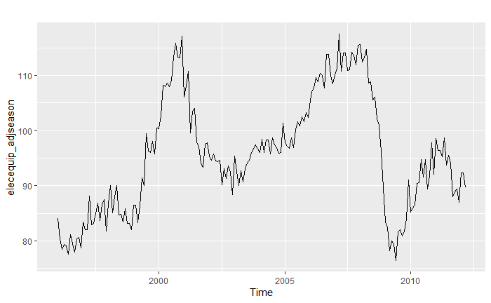
Note how by substracting the seasonal component, we have somehow achieved a smoother series, although clearly not stationary. Indeed, we can verify the resulting desasoned series’s ACF and PACF:
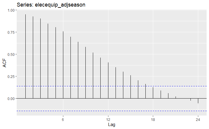
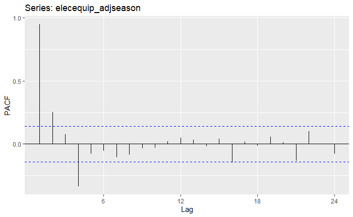
At first sight, we can see that this is clearly non-stationary. We can further confirm this with the ADF and KPSS tests:
How could we make this data stationary? We could try, for instance, differencing:
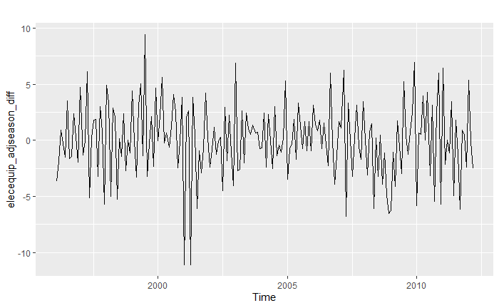
It looks like we “killed” some of the trend! All of sudden, everything looks significantly better:
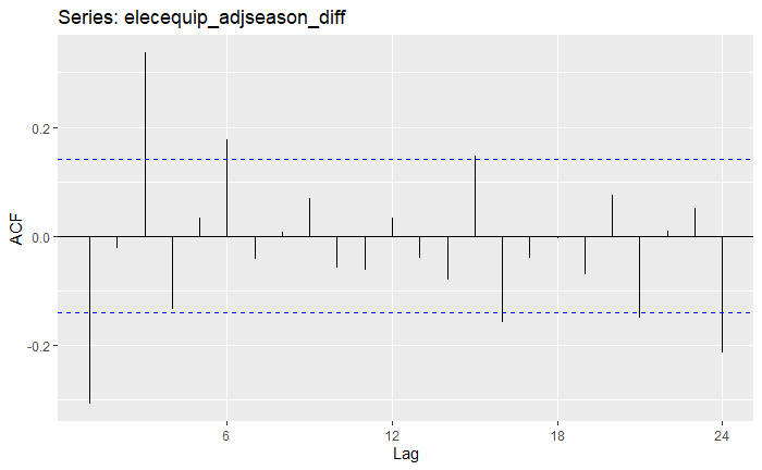
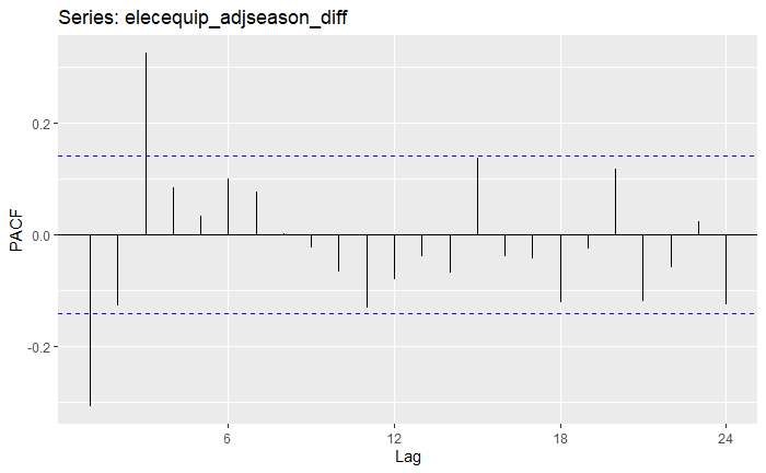
Although the ACF and PACF look much better, can we stay for sure that the data is stationary? Once again, we can run the ADF and KPSS tests to check:
Good news! In all cases, the tests seem to indicate that the resulting series is indeed stationary.
Fitting a SARIMA model
As we saw before, it looks like even after differencing the deseasoned process once, we obtain a seemely stationary process. Therefore, we could try to first fit an ARIMA(p,d,q) model using the auto.sarima function and see what we obtain:
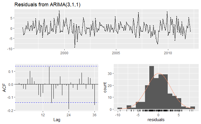
Indeed, we obtain an ARIMA(3,1,1) model, which implies that after differencing once, we would obtain a resulting ARMA(3,1) process. Let’s check the residuals and roots to assess whether the process is indeed stationary, causal, and/or invertible:
We can see that we indeed have a process that looks quite stationaryexcept for a couple of out-of-bounds lags. If this is indeed the case, by inspecting the roots we can see that it would also be a causal and invertible process. Let’s run a couple of additional diagnostics to confirm:
Indeed, the conclusions of both the ADF and KPSS tests seem to indicate that the process is indeed stationary.
Now, the question is, can we fit SARIMA process directly without de-seasoning first? Let’s try it out! Be sure to set the seasonal parameter in auto.arima as TRUE to ensure the search is done through seasonal components as well. Note that sometimes fitting seasonal models can be quite slow, so if you feel your machine is lagging, you can set the approximation argument to TRUE . In general, this will still produce a reasonable model based on the data at hand. In addition, you can also set the parallel=True , if your system enables parallelization through R. This will also speed things up, but you won’t see the trace.
And we obtain quite an interesting model! Namely an ARIMA(4,0,0)(0,1,1)[12] process. That is, a model with the following format:

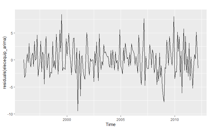
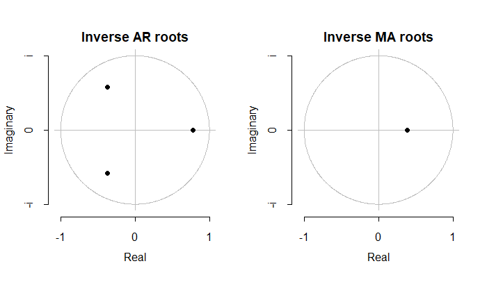
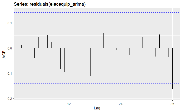
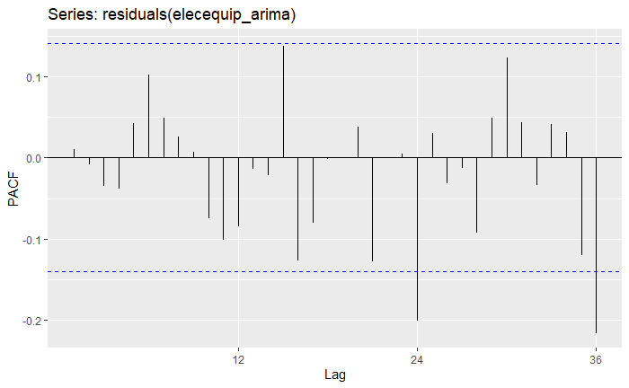
The usefulness in fitting such a model is that both trend and seasonality as pretty much taken cared of for us. Let’s inspect the residuals:
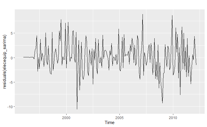
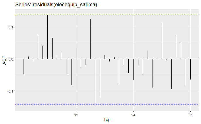
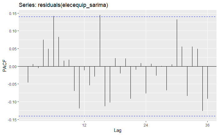
Indeed, we obtain an even better model than before! That’s because the SARIMA model is more complex than just simulating incorporating and removing seasonality, but it also takes into account ARIMA components based on seasonality alone, in addition to the base ARIMA ones. You can go ahead and run the other tests, and verify that the model is also causal (and obviously invertible).
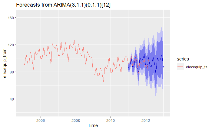
Finally, we are ready to make some predictions:
Very cool, eh?
Next time
And that’s it for this time! We are coming near the end of this article series on Time Series Analysis, and I take the opportunity to announce that I will be soon publishing a free-source book, with content almost identical to these series, including all the theory, examples, extra-appendices and much more! In the next article, we will be covering how to include exogenous variables into our analysis, that is, the so-called ARMAX, ARIMAX, and SARIMAX models. Stay tuned, and happy learning!


