
A Complete Introduction To Time Series Analysis (with R):: ARIMA models
In the last section, we discussed model selection for ARMA(p,q) models by using the AIC, AICc, BIC, which are metric functions based on the likelihood and the parameters, providing a certain measure that can be used to compare models against each other on the same data. In this article, we will now recatch the ideas of differencing and seasonality that we previously studied, and see how these can be integrated into the ARMA model. Let’s start by reviewing some essential concepts from the Differencing section
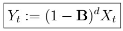
Differencing


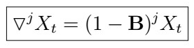
If you need a refresher, you can check this article, in which I discuss all of these in detail. The whole idea of having these operators is that we could essentially simplify some time series by eliminating some systematic trend component (and even some seasonality). How can we formalize this for ARMA(p,q) models?
Autoregressive Integrated Moving Average: ARIMA(p,d,q)


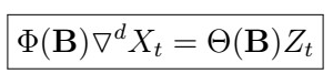
This formalizes the methods of differencing we saw previously under the Classical Decomposition model. In particular, we use the d-difference operator to eliminate trends (and in consequence some of the variances as we previously saw). This implies that the ARIMA(p,d,q) model can be used even for processes with a trend, although it is usually a good idea to remove it anyway!
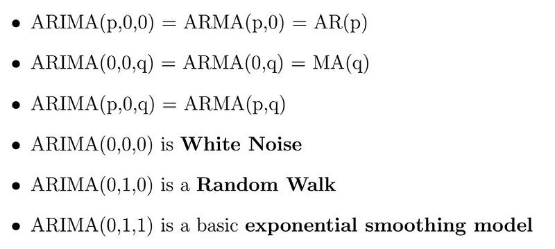
Trivial cases of ARIMA(p,d,q)
As you may guess, there are some equalities we can derive from the ARIMA(p,d,q) model:
Example: ARIMA(1,1,0)
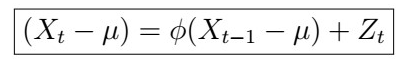
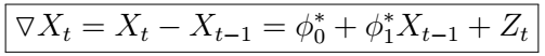
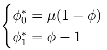
Let’s now make a concrete example: Let {X_t}~ARIMA(1,1,0). Then, this process has the form
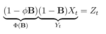
Now, what would happen in the case the phi coefficient is equal to zero, and in the case it is not?

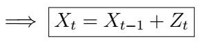
which is a Random Walk! , clearly not stationary. However, notice that
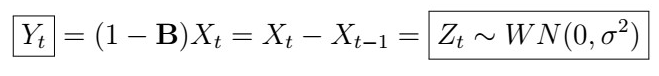
That is, by differencing, we achieve random noise , which is actually a stationary process.

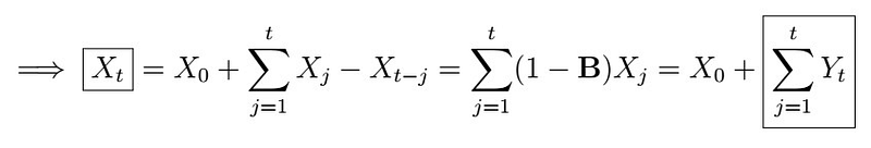
also, we have that
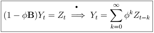
which follows as the process is causal. (See this article). Therefore, we can rewrite it as
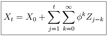
Once again, clearly X_{t} is not a stationary process as it is a random walk of AR(1) processes, however, we see that Y_{t} is!
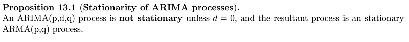
Stationarity of ARIMA(p,d,q) models
Proof idea
We illustrate for ARIMA(1,1,1) process, but the argument obviously generalizes for ARIMA(p,d,q). We can analyse the underlying Y_{j}’s if we take the difference:
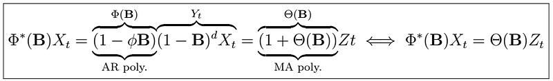
Here, let’s assume the AR(p) and MA(q) polynomials to have roots within the unit circle (see this article). However, the polynomial
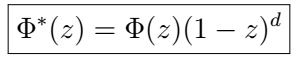
has d roots on the unit circle, so X_{t} is clearly not stationary.
Model Selection for ARIMA(p,d,q) models
Two approaches:
- Adjust the AIC/AICc/BIC to take into account the extra parameter.
- Test for unit roots.
The first one is identical to what we had considered in the previous article.

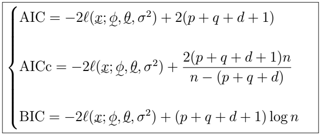
As you can see, this is not too different from what we had before. The model selection in this case is done the same way as before: select some criterion, try a bunch of models on the same dataset, and choose whichever model has the lowest metric. So far, this seems like a good approach. However, some statisticians argue that one cannot use likelihood-based methods, due to the differencing factor. Indeed, how can we test that our of choice of d is good, in particular? Instead, we will test for unit roots. The following two approaches are constructed based on that principle:
Intuition
Consider the (possibly) non-zero process

We can take the difference
, where
Therefore,
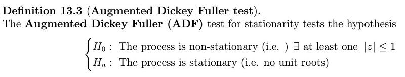
then X_{t} is non-stationary. The ADP test extends this idea to AR(p) polynomials.
Kwiatowski-Phillips-Schmidt-Shin (KPSS) test
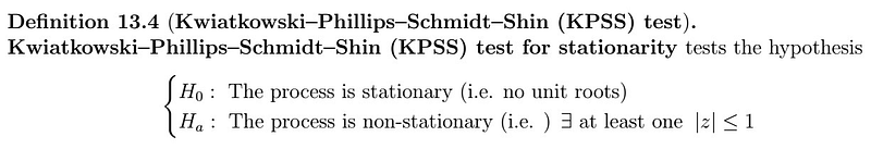
This test is quite similar in nature to the previous ones, except that the null and the alternative hypotheses are reversed. In addition, the null hypothesis actually indicates that the time sereis is stationary around a deterministic trend. This trend can be increasing or decreasing, but does not affect stationarity once removed. If you are curious, the original paper can be found here.
HowToR
As usual, we start by importing some packages:
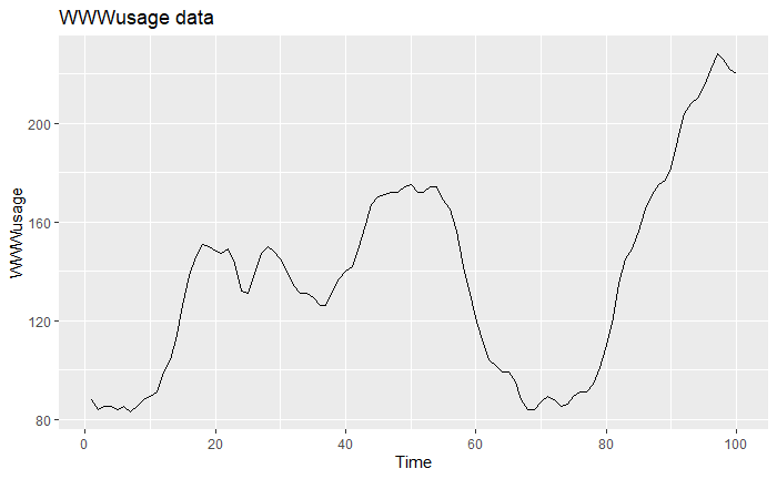
The data we will be using is the WWWusage data, available in R datasets (you don’t have to download it). This data itself is a metric for the extend to which people where using the internet in a period of time. First, let’s get a quick summary of the data:
We see that most values are between 99 and 168. Next, we can plot the data itself, along with its ACF and PACF:
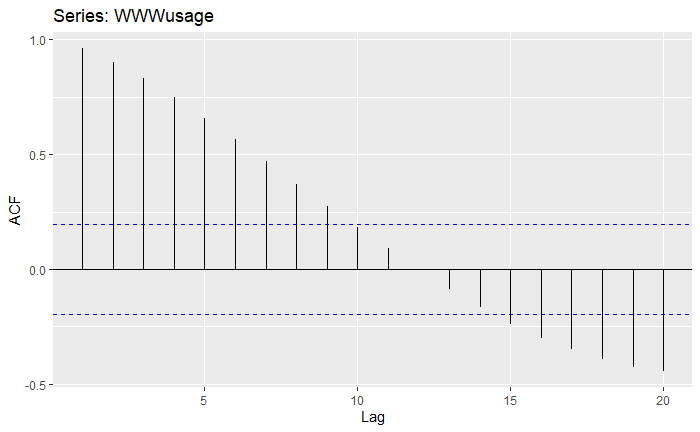
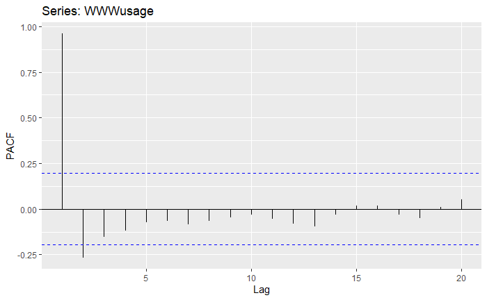
Right off the bat, we can see a clear indications of non-stationarity in the ACF, and strong partial autocorrelation for the first two lags.
As we fail to reject the null in the ADF test, and reject it in the KPSS test, this provides us evidence that the process is indeed not stationary. One thing we can try, is whether differencing and considering different lag orders used to calculate the statistic makes any difference.
We see that among all of these, only using lag-order=1 we reject the null. The problem is that we are not even sure which model this would be, as stationarity is concept almost proper to ARMA(p,q) models, as we saw previously. Therefore, by using this test on with respect to some fitted model, we must first assume the model indeed holds. We should then, make use of other stationarity tests, and keep these things in mind.
Fitting the model
The next thing to do then, is go ahead and fit some models. We will use the auto.arima function we saw in the previous article. Note that we set the seasonal argument to FALSE . Can you guess what would happen if we set it?
Notice how we obtained an ARIMA(3,1,0) model. That means, that if we were to take a difference once in the model, we would obtain an AR(3) model as a result. Let’s inspect the resultant model and its corresponding roots:
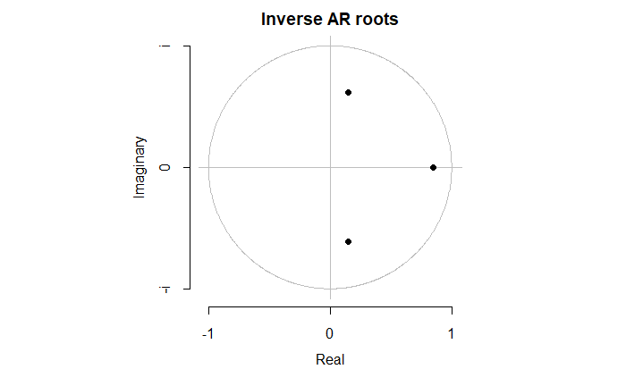
This tells us that after differencing, the model should indeed be causal and stationary, since the inverse roots all fall within the unit circle. We can verify this by applying the ADF test on the residuals as well:
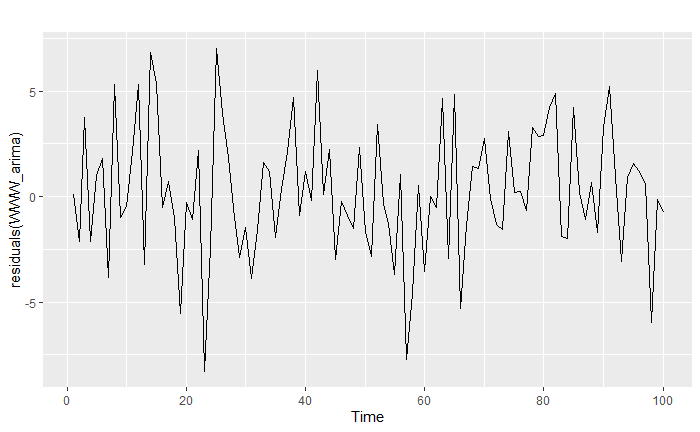
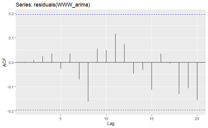
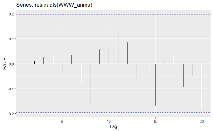
Similarly, plotting the residuals and their ACF and PACF functions take us to the same conclusion:
Note that we could also try enforcing a limit degree onto the auto.arima function, so that the polynomials or differencing components do not overpass that number. For instance, we can enforce d=2 , which will leave us with an ARIMA(2,2,0) as our best model:
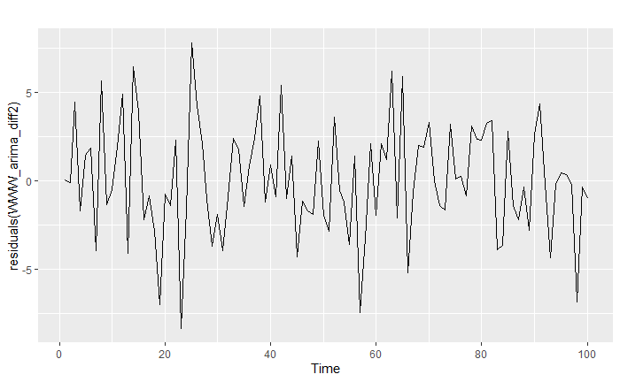
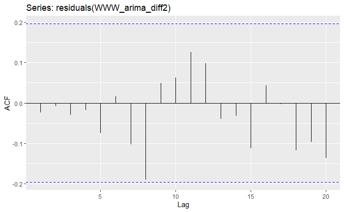
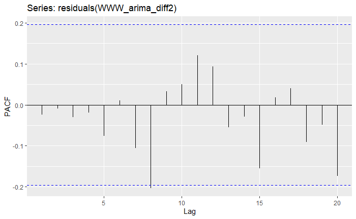
We see that in this case, the resulting model with double difference degree ARMA(2,2,0) is actually comparable in fit to the one we obtained before.
Next Time
And that’s it for now! In the next article, we will cover the so-called Seasonal ARIMA or SARIMA models, another useful extension in our Time Series models arsenal.


