
A Complete Introduction To Time Series Analysis (with R):: Estimation of ARMA(p,q) Coefficients (Part I)
In the last article, we discussed the extension of the Innovations algorithm for the more general ARMA(p,q) process, which allowed us to make predictionsf for arbitrary number of timesteps in the future. However, we still haven’t seen how to estimate the actual ARMA(p,q) model coefficients. In this article, we will see two algorithms for estimating AR(p) coefficients, and in the next article, we will see how to estimate MA(q) and start taking a look into jointly estimating ARMA(p,q) coefficients. Let’s jump right into it!
Estimation of AR(p) :: Yale-Walker
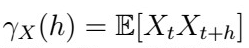
In real world problems, the ACVF is the easiest thing to estimate using the sample data. In other words, recall that we can estimate it as
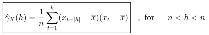
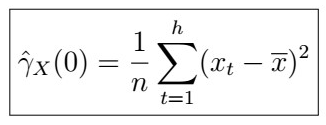
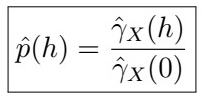
From which we can in turn estimate autocorrelation as
The Yale-Walker equations rely on the method of moments, to construct statistics that help us estimate such coefficients.
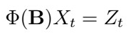
Consider the AR(p) process with coefficients
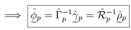
Then, it’s estimated values (hat phi) satisfy the equations
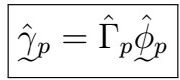
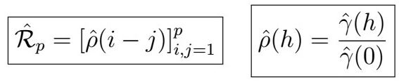
where

Here, recall that the big Gamma matrix is symmetric with all correlations between 0 and (p-1), and the other vector is the gamma vector of all correlations from 1 to p. Further, this allows estimation of the variance as
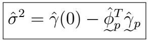
, where
Moreover, for large n and given a “true” AR(p) model (that is, given that p is correctly specified)
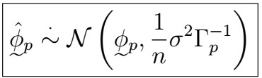
That is, the parameters follow a multivariate normal distribution as specified above.
Proof
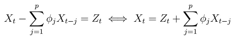
Recall that for a mean-zero process,
. If our process is AR(p), then
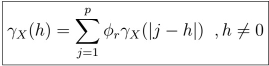
That is, we have that
From this, it follows that
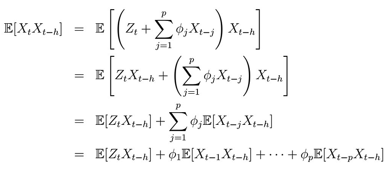
This implies that
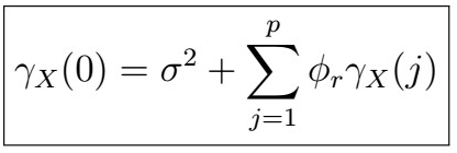
Differently put, we have a system of p linear equations with p variables; we can use these to solve for the phi coefficients. Written down:
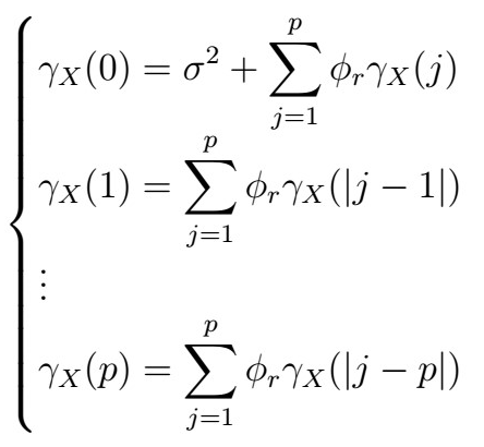
Note that the first equation is independent of the others! Therfore, replacing the sample ACVF versions and writing down in vector notation, we see that this becomes
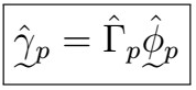
And therefore we can estimate the coefficients by solving for the phi vector, as stated.
Remark
Suppose that the true model is an AR(p) model, but instead we fit an AR(m) model, where m<p. If this happens, there will be missing coefficients from the true model, and so the estimated coefficients will no longer be (statistically) consistent! On the other hand, if m > p , then we can write
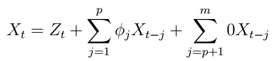
, so that the extra parameters we specified are set to zero, and the model still recovers the true AR(p).
Burg’s Algorithm
Recall that the PACF is given by
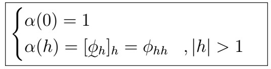
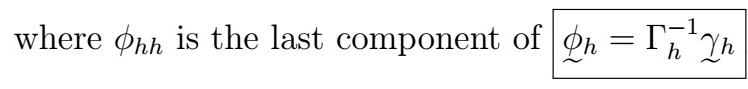
wher the Gamma matrix and vector are given by
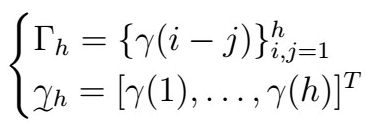
Recall that the PACF tells us how much of the variablity in our value at time t is explained by a value at lag p, if we are fitting the BLP with t components. If we have a causal AR(p) model, then
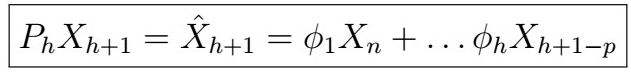
The idea is as follows: we can also use the PACF to estimate the AR(p) coefficients. Burg’s algorithm makes precisely use of this.
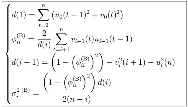
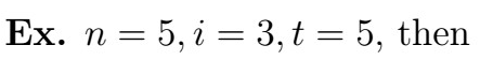
Consider an AR(p) process.
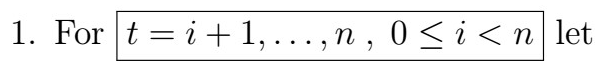
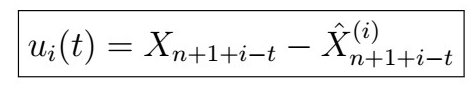
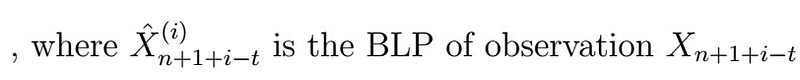
given the previous i observations.
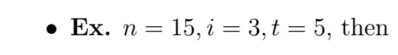
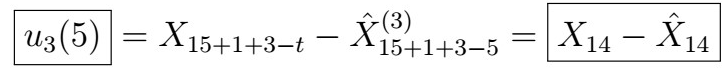
, where

Note that for each i , we are looking at the innovation that we get from taking the BLP using the previous i observations for looking at a particular time in our sequence; i.e. it works us backwards from the last time point all the way back to the earlierst point we can go by i observations.
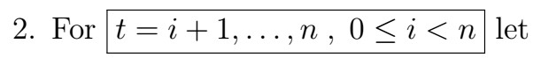
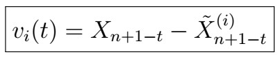

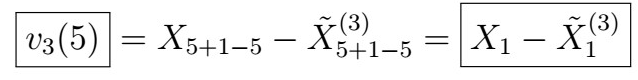
where

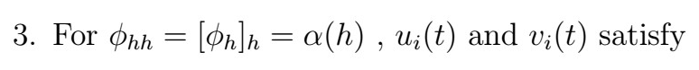
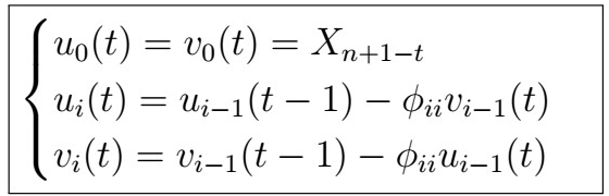
Note that both u and v are functions of the data and phi parameters!

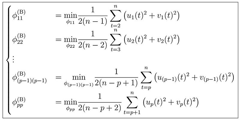
In addition, we use

You can think this as estimating the coefficients optimizing (minimizing) a mix between averaged adjacent past and future observations for every time step, and considering these in turn.
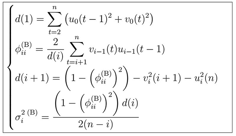
6. Although the proof is definitely out of scope, with this we have actually estimated a set of PACF coefficients
Which are valid up to step p. At this point, we essentially go back to the Durbin-Levinson algorithm , that is, for n steps, we
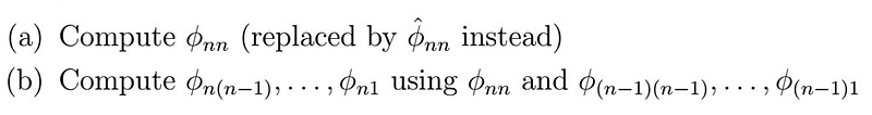
7. This yields in turn a set of coefficients which can be used as estimations of
That is, the last value of the phi values at each timestep, which constitute the set of estimated AR(p) coefficients.
8. For large n and given a “true” AR(p) model, it holds that
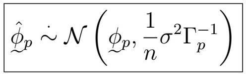
This asymptotic normality ensures “nice” properties when it comes to confidence intervals
And that’s pretty much it! Although it might be somehow confusing due to the notation and the various formulas and equations, the basic idea is that Burg’s algorithm produces a set of somehow more statistically sound estimates of the AR(p) model (assuming this one has been correctly specified), by considering not only projections and BLP that use observations from the past, but also even in the “future”, given the data at hand.
How to R
As usual, we first start by importing a couple of useful libraries.
Estimating AR(p) coefficients
We will first start by creating some artificial AR(4) process along with some data generated from it, and then proceed to use the algorithms we have seen to estimate its coefficients. First, let’s generate some data:
Now let’s check the roots of this process to make sure it is stationary,
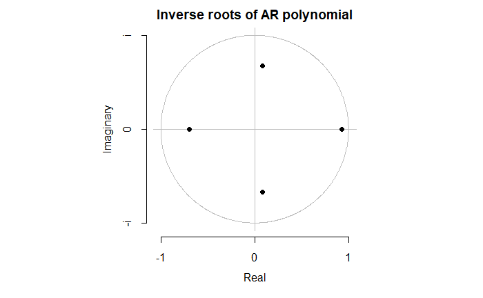
So we see that we have all four different (inverse of the) roots that are all inside the circle, so the process is causal and stationary. (Although see that one of them is close to the edge!!! That is, although the process is stationary, the hardest the estimation will be, the bigger the variance, the worse the performance). Now generate some data and compare sample ACF and PACF to truth
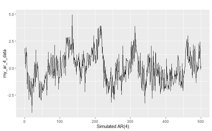
This definitely doesn’t look like white noise! Let’s check its ACF and PACF functions:
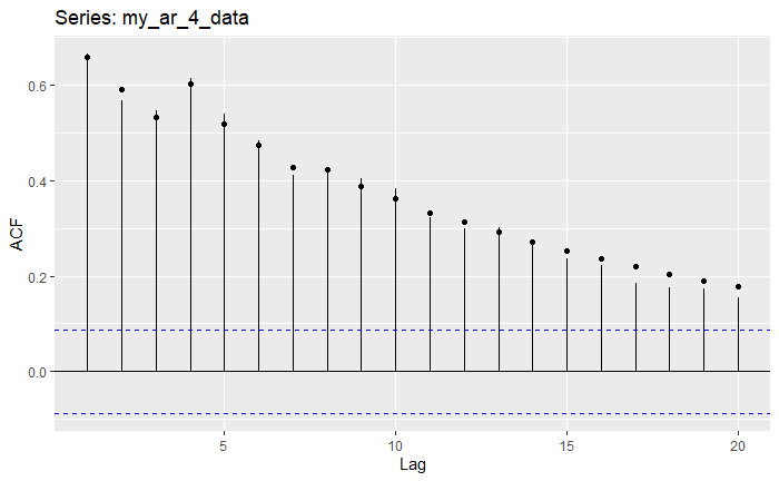
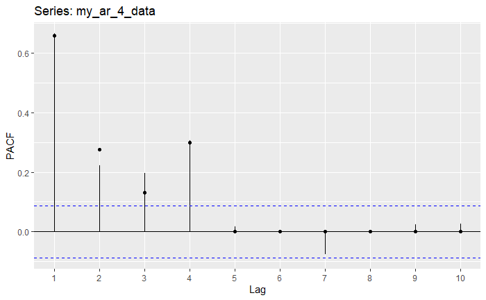
Notice how the number of lags that fall out of bounds is precisely 4; the specified degree of the AR(4) polynomial. In the code above, we have also plotted the actual values (as points). Also, notice how close the estimated ACF and PACF values are actually are to the true ones.
Let’s now try to fit a couple of algorithms with the help of the ar function:
In the first part of the code block, we fit three models: Yule-Walker, Burg’s Method, and the Gaussian Time Series MLE. Then, we construct a function to pack to repeat this process and also pack all the relevant information we need into one big tibble object. We can then check the tables with information about the true and fitted coefficients and standard errors as follows:
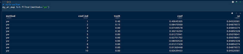
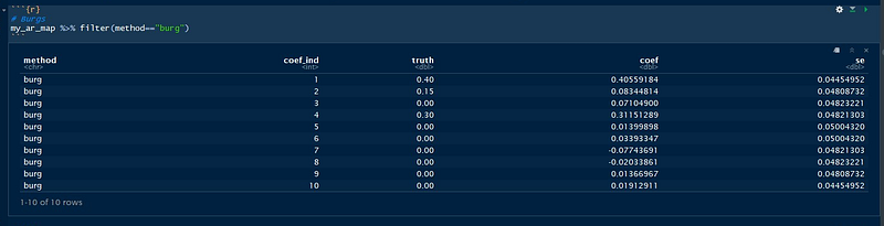
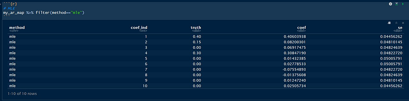
Notice that even though we over-specified the model, the extra-coefficients are actually very close to 0! In general, it’s better to “over-specify” the model, but we will see later a simple, but solid method for model selection.
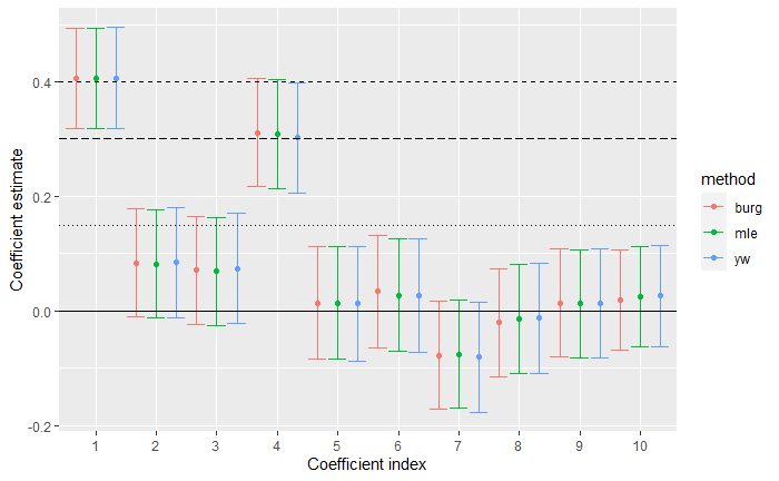
Let’s now go and visualize the actual coefficients and confidence intervals that we obtain from the tables for the different methods:
Now, we would like to obtain some diagnostics with the model; we can also use the Arima function to fit an AR(4) model using MLE, and obtain diagnostics.
That is, we explicitly specify the order of the model, and then we can see the corresponding estimated coefficients, the sigma², log-likelihood, and other evaluation metrics. Checking the residuals yields
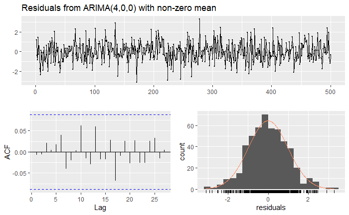
From which we can see that the model indeed looks like white noise, and also approximately normally distributed. The Ljung-Box test does NOT reject the hypothesis that the residuals are white noise.
Next time
In the next article, we will continue with algorithms to estimate the MA(q) coefficients independently, then how to combine these along with the other AR(p) algorithms to estimate the ARMA(p,q) coefficients as a whole, and finally, we study Gaussian Time Series in subsequent articles, one of the most widely used assumptions to estimate ARMA(p,q) parameters. Until next time!
Last time
Forecasting with ARMA(p,q) models