A Complete Introduction To Time Series Analysis (with R):: Estimation of ARMA(p,q) Coefficients (Part II)

In the last article, we learned about two algorithms to estimate the AR(p) process coefficients: the Yale-Walker equations method, and Burg’s algorithm. In this article, we will now see a very simple way to determine the MA(q) process coefficients, and a first approach to estimate the ARMA(p,q), jointly. Let’s see how this works:

Estimation of MA(q) (Innovations)

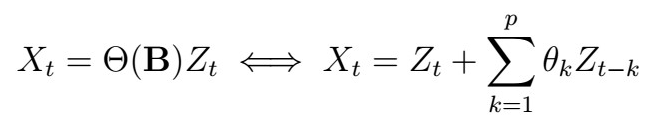
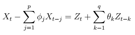
As you may guess by the title, the way to estimate the MA(q) coefficients is… the Innovations Algorithm we saw before. Recall that the MA(q) process can be written as

The idea is as follows:

• Recall that during the iterations of the Innovations algorithm, we obtain the Theta matrix

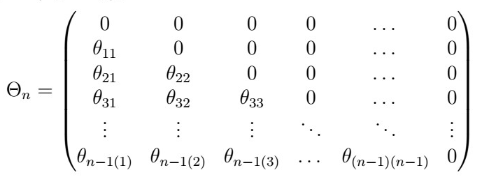
which in turn provides the coefficients used in the recursive Innovations formula:

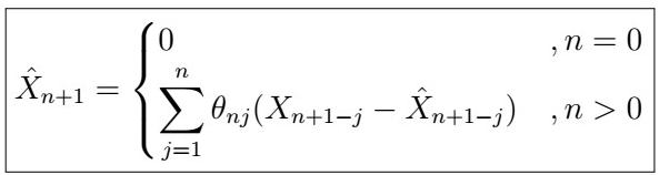
. It turns out that these are actually also consistent estimators of the MA(q) process coefficients!

• We can then apply the Innovations algorithm by substituting the sample ACVF instead of the actual ACVF, that is

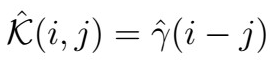
, and thus obtain, at the m-th step, a set of coefficients

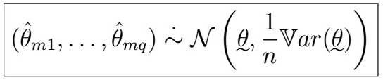
• It can be shown that for sufficiently large m

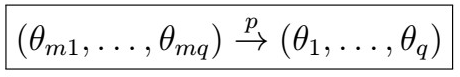
That is, the estimates converge in probability to the true MA(q) parameters.

• Further, it can be shown that for large m

Estimation of ARMA(p,q) — Hannan-Rissanen Algorithm

So far, we have come up with methods to independently estimate AR(p) or MA(q) coefficients, but not yet a way to estimate both together. The Hannan-Rissanen algorithm does precisely this. The idea is as follows:

1. Consider only the AR(p) part of the model, that is, assume

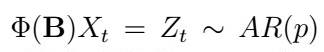
, and estimate its coefficients using the Yule-Walker equations or a combination of Burg’s algorithm + Durbin-Levinson.

2. Use the resulting AR(p) coefficients to estimate the White Noise process

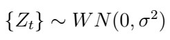
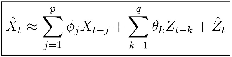
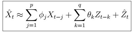
3. Now, recall that the ARMA(p,q) has the form

Using step 2), this implies that

4. Using this estimation, we can now use Multiple Linear Regression to find suitable parameters. That is, we use least squares to solve the Sum of Square Residuals (SSR) given by

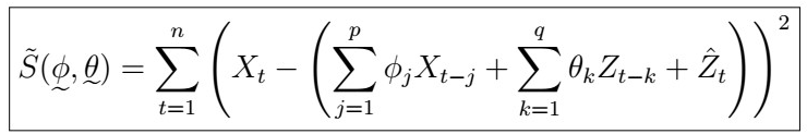
, on parameters phi and theta of interest, which will be the final estimated coefficients for our ARMA(p,q) model at hand :). If you are a bit rushy on Linear Regression, check this article for a refresher!

Moment Estimators

We have now seen a variety of methods to estimate AR(p), MA(q) or ARMA(p,q) coefficients by using either the ACF or PACF:

1. Yule-Walker for AR(p) (ACF)
2. Burg’s algorithm + Durbin-Levinson for the AR(p) (PACF)
3. Innovations algorithm for MA(q )(ACF)
4. Hannan-Rissanen for ARMA(p,q) (ACF/PACF + MLR)

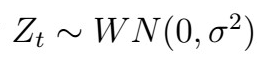
Problem: Although all of these algorithms are quite elaborated and produce theoretically consistent parameter estimators, in practice, we have trouble getting a small asymptotic variance. In other words, these tend not to perform so well in all datasets! especially when the true model is misspecified. In such cases, non-linearity can produce rather bizarre results and overall poor fit. Often, we also require a large n (number of observations) to obtain useful results, but due to the nature of Time Series data, sometimes data might be limited. Therefore, we would like to add another assumption: specifying underlying White Noise as Gaussian. We will explore this in the next article :).

How To R

As usual, we first start by importing a couple of useful libraries.

Estimating MA(q) coefficients

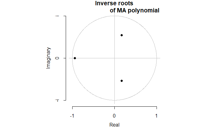
This time, we will use the Innovations Algorithm to estimate MA(q) coefficients. Let’s start by simulating some data, and checking its roots to verify invertibility:

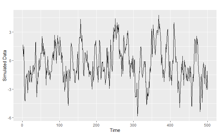
Now we can go ahead and generate the actual data.

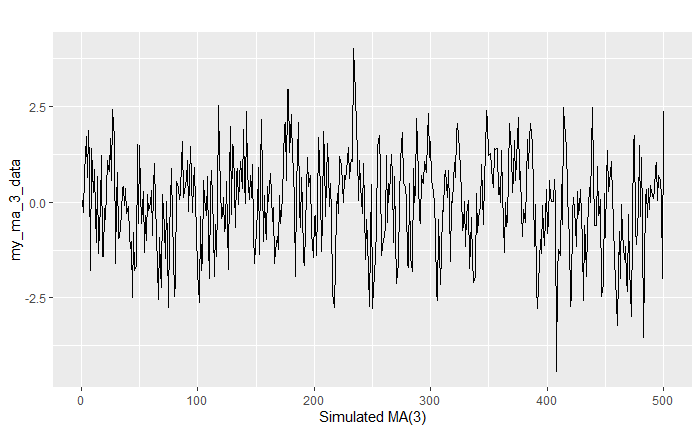
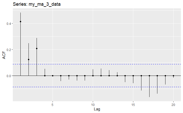
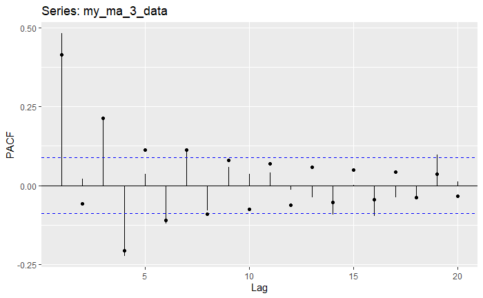
Note how here, the ACF shows three points that fall out of bounds, exactly the MA(3) specification. The PACF shows more than 3 points out of bounds, but notice how only three of them are quite far from the bounds themselves, as we get this oscillating but decreasing behavior. Let’s now use the Innovations Algorithm itsmr::iato estimate the coefficients, and then another function to pack them together to visualize the progression of the estimation along with confidence bounds for every point. The code for this is quite complex, so it’s not essential that you understand what’s going on, but I left some comments regardless.

Now the visualization:

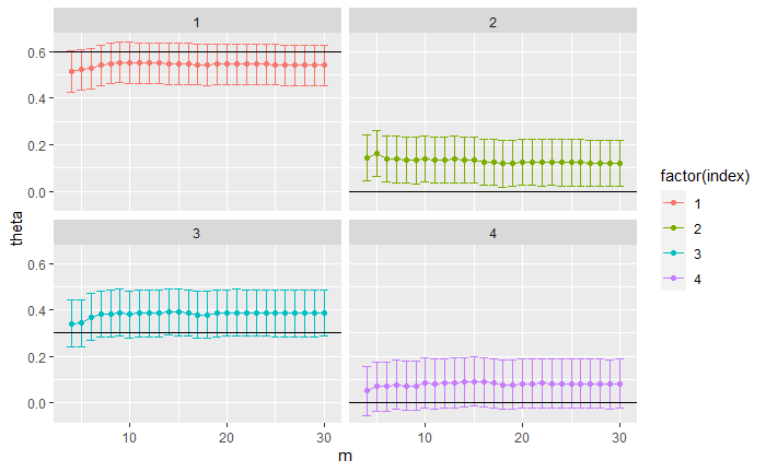
Now, remember that the true coefficients we specified c(0.6, 0, 0.3, 0), yet here we even seem to have an extra coefficient and the estimated second coefficient is also quite far from zero! As we mentioned before, the problem with using the Innovations algorithm alone is that we need a lot of data and iterations for it to yield good estimates. You can try and repeat this experiment, this time with m=1000 instead of 500, and see how this helps to improve the estimations. Let’s fit an MA(4) model (with Gaussian MLE, which we will see in the next article) to verify the residuals.

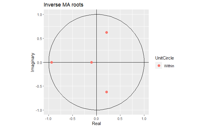
We see that this time the coefficients are much closer to the actual ones: that is c(0.6, 0, 0.3, 0). Inspecting the roots, we see that although we do have the extra coefficient one, this one actually lies very close to the boundary.

Checking the residuals:

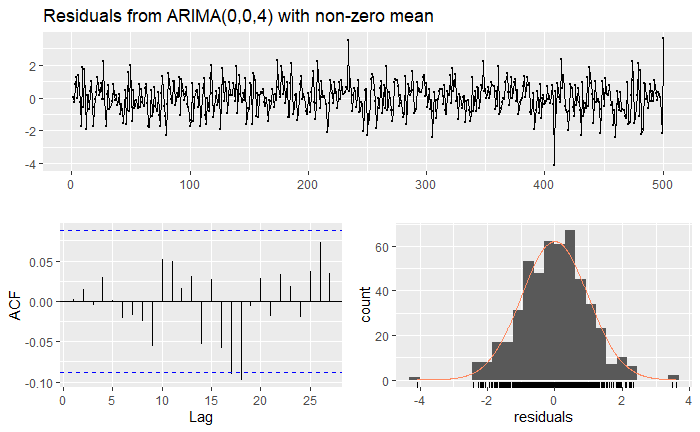
Which indeed are proof of a stationary time series.

Estimating ARMA(p,q) with Hannan-Rissennan

Let’s generate now some data for an ARMA(2,1) model:

As usual, let’s visualize our data:

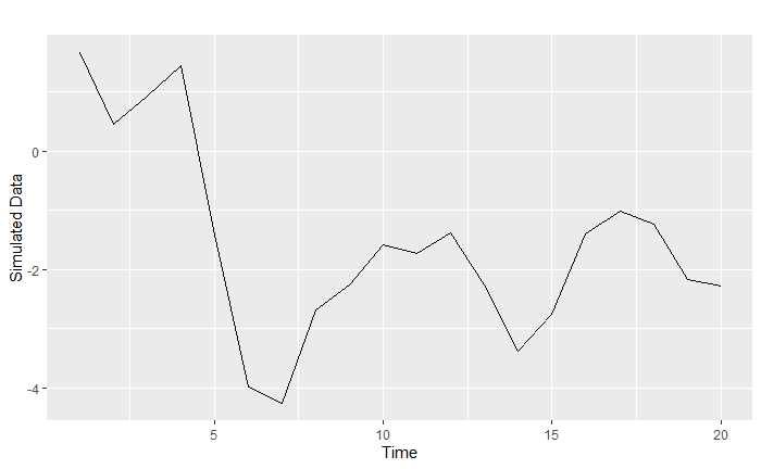
Once again, you see that it’s actually pretty hard to figure out what to fit the method. In order to apply this algorithm, however, we have to make sure our series is a zero-mean process. We this as follows:

Recall true values were AR(0.6,0.2) and MA(0.4), these are not very close! Let’s compare this to the MLE estimates:

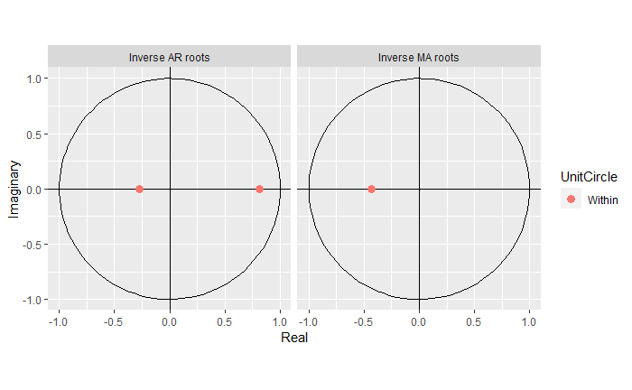
Notice that these are much better estimates. We can see that the estimated roots also provide proof of stationarity, causality, and invertibility:

Finally, let’s inspect the residuals:

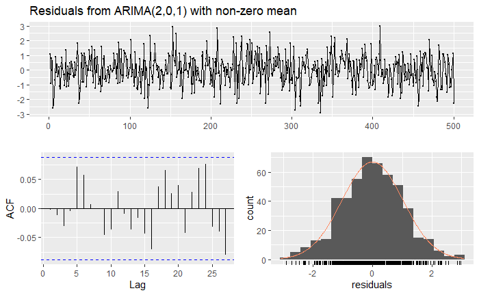
These all seem to indicate stationarity, as well as normality of the residuals, and an apparent White Noise process. To compare both algorithms, we will first create a tibble object:

Now we compare with larger values of n with a modified version of the Hannan-Rissennan algorithm, which does not compute sigma square. Don’t worry about understanding the code itself.

Using this fact function, we can go and refit the data again:

Next, let’s verify the roots:

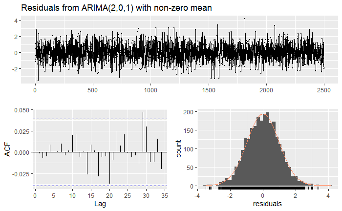
And the residuals:

Once again, let’s compare the coefficients:

We see that now, after running Hannan Risannen with a larger sample size, the estimated coefficient are a bit better than before, but they still do not beat the MLE. This doesn’t mean that Hannan-Rissanen is completely useless, in fact, we can use it to initialize the MLE coefficients, which will ensure faster convergence.

Last time

Estimation of ARMA(p,q) Coefficients (Part I)

Next Time

Gaussian Time Series

Main page

Follow me at

1. https://www.linkedin.com/in/hair-parra-526ba19b/
2. https://github.com/JairParra
3. https://medium.com/@hair.parra