Why Extremistan Must Have Less (Minor) Volatility Than Mediocristan

Note: Taleb has likely included about dozen different simplified, non-mathematical explanations of what I am going to explain here throughout all volumes of the Incerto, so if you want a non-mathematical explanation, you can go find one he has written. This article requires the understanding of basic probability 101 level information. I am also assuming that you are already aware of Taleb’s terms Mediocristan and Extremistan, and you either already know what they mean, or you think you do!

I am a huge fan of Nassim Taleb’s Incerto, an extended essay on uncertainty and opacity which includes Fooled By Randomness, The Black Swan, The Bed of Procrustes, Antifragile, and Skin in the Game. I listened to the audio versions of each of them (besides The Bed of Procrustes) at least 4 times all the way through now, and I am currently slogging my way through Volume 1 of Taleb’s more mathematically rigorous version of The Incerto which he calls the Technical Incerto right now.

Because of how much time I have spent pondering his major works over the years, I am in a relatively good position to observe the concepts put forth throughout his books which most people who read 2 or 3 of his books once never quite understand. That is what this brief article is about, one of the most fundamental lessons of all of his books, namely, the fundamental differences between Mediocristan and Extremistan, i.e. mild-type randomness vs wild-type randomness (or Gaussian versus Power Law if you prefer).

The Question

In order to know whether you too have fallen for this extremely common (according to Taleb) misunderstanding of the difference between Extremistan and Mediocristan, answer the following question:

When a system, phenomenon, environment, economy, or other type of random process transitions from Mediocristan to Extremistan, would you observe this shift as a greater or lesser amount of moderate volatility (by moderate, I mean variation from the observed mean which is less than 1 mean absolute deviation, median absolute deviation, or root mean squared error away)?

In other words, how would it change the empirical rule for the distribution? Remember, for a Gaussian distribution, the empirical rule is that about 68% of all observations will fall within 1 root mean squared error (denoted here, as always, by the lower case version of the Greek letter sigma), 95% within 2 RMSEs, and 99.7% of all observations within 3 RMSEs (I try to avoid calling the Root Mean Squared Error the Standard Deviation at all times, to see why, check out my article MAD > STD):

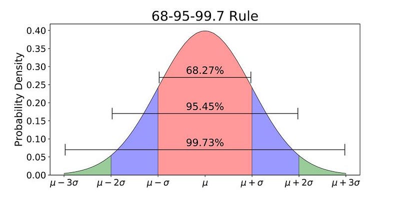
Obviously, if you are aware of what Taleb means by Mediocristan and Extremistan, and you know what a Gaussian Distribution is, then you know that it is the quintessential example of Mediocristan. Thus, the question becomes this: Would the percentages of the observations included within 1 root mean squared error (from its mean) of a distribution with fatter/heavier tails have a higher or lower percentage than the Gaussian does, i.e. greater than 68.27&?

According to Taleb, most graduate students in mathematics who he asks this question to verbally give the wrong answer.

The Answer

The percentage of observations within +/-1 sigma goes up!

Despite listening to every volume of the Incerto several times when I first came across this question (because I found it in either a video on Taleb’s YouTube channel, one of his papers, or an online article explaining some of the findings in his technical papers, and NOT in any of the volumes of the Incerto), I got the wrong answer so don’t feel bad if you did too.

But now that I know the answer, it is clear that it really is said in a multitude of other ways throughout the Incerto. The first example that pops into my mind is the vignette towards the beginning of Antifragile about the two brothers from Cyprus living in London where one of them drives one of the famous London ‘black’ caps, and the other works at a bank. In that vignette, the brother who is a cab driver feels bad because he thinks his job is not as consistent or predictable as his brother’s salaried position, but he is mistaken.

The Mathematical Explanation

Quick probability refresher:

1. All probability distributions have a cumulative/total area under the curve of 1, that means all 4 of these curves, and any other possible curves representing distributions must all have the same area under them which is 1.
2. Kurtosis is the name for a common measure of how heavy the tails of a given distribution.
3. A Gaussian distribution is said to be mesokurtic, a distribution with thinner tails than a Gaussian is said to be platykurtic, and a distribution with fatter tails than a Gaussian is said to be leptokurtic.

I first came across this question, made my wrong guess, then learned the right answer years ago, and I have never forgotten it, but the mathematical reason why never struck me until last month when I saw this graph in Volume 1 of The Technical Incerto: The Statistical Consequences of Fat Tails:

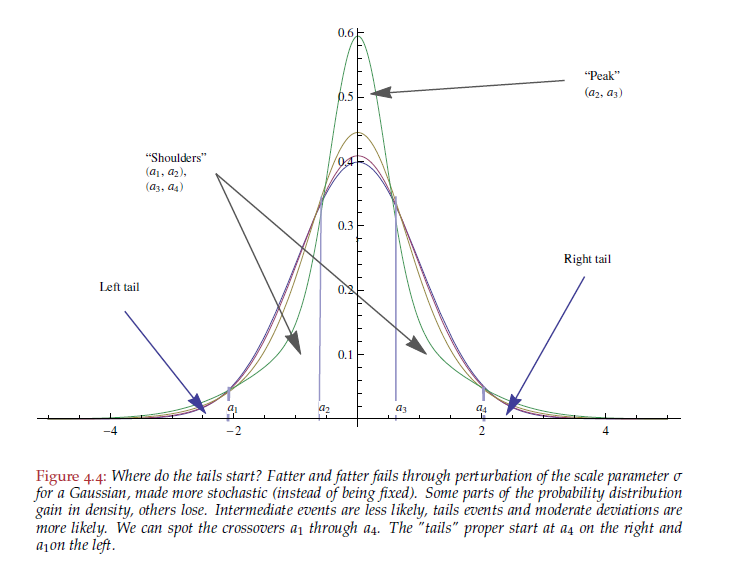
What this graph shows is 4 different probability distributions which each have differing levels of kurtosis. The tails of all of them begin at the points Taleb indicates, notice that the peaks (the height at and right around their means) are higher and higher for the distributions as their tails get fatter and fatter (which you can see by how slowly their y-axis values continue to descend beyond the starting point of their tails where the ones descending more slowly have fatter tails). This is simply another way of stating the answer to the question earlier, i.e. the more kurtosis a distribution has, the fewer minor variations it has.

I truly hope all of this has been a good setup for my recent epiphany, and here it is: the fact that the tails are fatter means they have more probability mass in them, so that extra probability mass has to come from somewhere else besides the tails to maintain a total probability mass of 1!

In the limit, the distribution with the fattest tail would a distribution which looks like a uniform distribution over a very large number of observations for a very long time with just one large extreme deviation at some point, and never again thereafter. Adding a second large deviation would necessarily decrease the magnitude of the first deviation by its own magnitude exactly.

Another Graph Just for Good Measure

Just in case you still don’t quite get it, I also include Figure 2 from the pdf supplement to my audio version of Antifragile on Audible here:

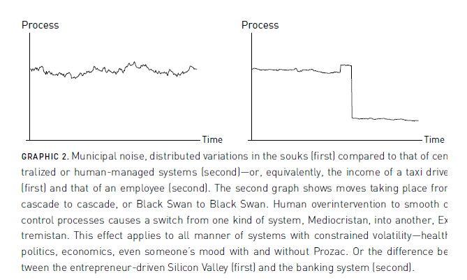
As you can see, the daily, weekly, monthly, quarterly, and yearly variations in the process are much smaller in Extremistan. And that is why Extremistan is so dangerous, because the dangerous catastrophic shock to the system is not present in the data, so a naive analysis of the data cannot let you know it is even possible!

The end.

More Articles from Me Like This

I have written several other articles on my Medium blog explaining technical concepts from Nassim Taleb’s Incerto or inspired by things I have learned from his YouTube tutorials and/or online articles, including:

1. Blindspots in the Standard Risk and Decision Theory Curriculum
2. Sometimes, the Difference Between a Test Which is “Statistically Significant” and one Which is “Not Statistically Significant” is Not Itself Statistically Significant
3. An Introduction to Nassim Taleb’s 4 Quadrant Model and The Law of Medium Numbers, Part I
4. An Introduction to Nassim Taleb’s 4 Quadrant Model and The Law of Medium Numbers, Part II
5. Stop Referring to the Gaussian Distribution as the “Normal” Distribution
6. Mean Absolute Deviation vs “Standard” Deviation