An Introduction to Nassim Taleb’s 4 Quadrant Model and The Law of Medium Numbers, Part I

Motivation for this article: I took a graduate level course on decision & risk analysis in the Systems Engineering department as an elective in the Spring semester of 2022 during my master’s program in Data Analytics Engineering at George Mason University. The material, in the lectures, in the homework, and in the textbook, was painfully, and dangerously out of date.

I was told I could do a solo final paper for the class after missing the deadline to join a team for a group project due to a temporary health emergency, and after being alarmed at how out of date some of the material still was given my knowledge and admiration of the work in Risk and Decision Theory by the loveably cantankerous Nassim Nicholas Taleb, so I asked my professor if I could write a long paper explaining the updates to the curriculum of the course itself I strongly feel should be made and he was intrigued enough by my moxy in asking him to do so that he agreed.

At least 85% of this is article is that paper, but some corrections have been made and extra explanations and clarifications added on as well. To my knowledge, the curriculum was not changed at all subsequently, but I did at least get an A despite calling the entire course outdated.

Overview

This research report for SYST 573 — Decision and Risk Analysis presents underappreciated problems that arise when real world risk analysts and decision makers commit the error of relying too heavily on idealized versions of standard statistical, machine learning, or econometric modeling and forecasting techniques without understanding when these methods of analysis work the way academic textbooks claim they work (in Large samples or Asymptotically, but fail to provide any guidance whatsoever on how to know where your sample is large enough across all possible types of underlying probability distributions).

It then goes on the provide alternative heuristics and decision-making guidelines you can rely on when you don’t know if your sample or source data is large enough to justify direct application of classical elementary notions of statistical inference in the decision-making context you are faced with.

After that, analytical justifications and graphical explanations are provided to demonstrate exactly why most sophisticated analytical modeling and forecasting methods are valid much less often than most people, including applied statisticians and data scientists realize. This error has been identified in the literature as The Law of Medium Numbers, and the final part of this report highlights its relationship with the already well understood error known as The Law of Averages.

Part 1: Nassim Taleb’s Four Quadrant Model — A Map of the Practical Limitations of Statistics in the Real World

1.1 Introduction, Motivation, and Purpose of this Article

Most of the new concepts, categories, and decision making guidelines discussed in Part 1 of this report comes from the peer-reviews journal article, Nassim Taleb’s landmark 2009 paper “Errors, Robustness, and the Fourth Quadrant,” which was written by the maverick probabilist, former options and financial derivatives trader, risk taking theorist, and fragility/antifragility theory pioneer, Dr. Nassim Taleb (who has been a quarter time Distinguished Professor of Risk Engineering at the NYU’s Tandon School of Engineering since September 2008 when he retired from his long career as an options trader), and published in 2009 in the International Journal of Forecasting.

I’ll start off with a quote from the paper itself:

“The extensive literature on decision theory and choices under uncertainty so far has limited itself to [1] assuming known probability distributions (except for a few exceptions in which this type of uncertainty has been called “ambiguity”, and [5] ignoring fat tails. This paper introduces a new structure of fat tails and classification of classes of randomness into the analysis and focuses on the interrelation between errors and decisions.”

The new framework introduced in the paper partitions types of decisions along with their corresponding exposures to unforeseen (and often unforeseeable) risks into four different categories, or “Quadrants,” by dividing them into two qualitatively and quantitively distinct types of decisions in terms of the possible payoffs which result as a consequence of those decisions along two different dimensions (qualitatively different levels of randomness), leading to a total of four mutually exclusive and collectively exhaustive “quadrants.”

(i) The Two Types of Decisions by Payoff

The first type of decisions are simple decisions with only binary potential payoffs. For these simple decisions with binary payoffs, the only matter of concern is whether your belief, claim, or prediction is True or False, there is no such thing something being “very true” or “extremely false.” So, for instance, if you are a fertility doctor seeing a female patient who wants to know the results of a pregnancy test you had her take recently, the only possible results of that pregnancy test are Positive, indicating that she is pregnant, or Negative, indicating that she is not pregnant, she can’t be “very pregnant” or “very not pregnant.”

For these types of decisions, all that matters is the probability that the events will happen, not on their magnitude. While very easy to deal with, unfortunately, this type of decision is not very common in everyday life either as a common citizen in personal matters, or as a decision maker, or stakeholder at a firm. A few examples of this type would be placing a bet on the outcome of a democratic election or a fixed bet on the outcome of someone flipping a (fair) coin, or perhaps laboratory experiments of hypotheses by researchers.

The second type of decisions are those subject to complex potential payoffs. The Decision Maker does not (or at least, he need not) care about how frequently the predictions on which he bases his decisions are accurate, but about the impact or magnitude of the payoffs, and the cumulative effect of the interaction between the overall accuracy rate of the predictions made during the process of making many decisions over time multiplied by the magnitude of the payoffs received or penalties incurred as their consequences.

These payoffs depend on higher moments of the underlying distributions. Put more simply, when one invests, he cares not about the frequency of the momentary increases or decreases in the value of that investment; instead, he cares about their overall expectation, i.e., how many times the value increased or decreased multiplied by the corresponding magnitudes of each of those increases and decreases. In extreme cases of type 2 decisions, as Taleb puts it, “One can be right 99% of the time, but this does not matter at all, since with some skewed distributions, the consequences of the expectation of the 1% error can be too large.”

(ii) The Two Probabilistic Domains

Most statisticians, whether applied or theoretical, when they divide up different probability distributions into groups of related distributions, they do so in terms of what refer to as families of probability distributions (e.g. the Gamma family, Exponential family, Gaussian family, etc.). However, the motivation behind these categorization schemes are purely mathematical considerations, such relationships between distributions in terms of having shared shape or location parameters and the like, but these families are not very practically useful for Decision Analysts or Decision Makers.

That crucial practical gap was Taleb’s fundamental purpose for his Four Quadrants paper. His novel categorization scheme for probability distributions intended for practical purposes by Decision Makers, not Ivory Tower professors who never decide anything important, divides all of them into one of just two different domains. These two domains are quite distinct qualitatively, quantitatively, and practically.

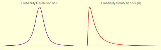
The first probabilistic domain is the class of all probability distributions subject to what he calls Type-1 Randomness, which includes all probability distributions which are “benign” in terms of their kurtosis. A particular probability distribution which has only a mesokurtic shape profile, that is, its overall kurtosis is close to 3, therefore, its excess kurtosis is close to 0. they have thin-tails and are nonscalable. In his popular books (Fooled By Randomness, The Black Swan, The Bed of Procrustes, Antifragile, and Skin in the Game), Taleb refers to this probabilistic domain as Mediocristan.

The second probabilistic domain includes all probability distributions subject to what he calls Type-2 Randomness. The second domain is that which is includes all probability distributions which are significantly leptokurtic (a higher 4th moment than the Gaussian), i.e., they have thick-tails or a long-tail (often referred to informally as “fat-tails”) and are scalable (or even fractal). In his popular books, Taleb refers to this probabilistic domain as Extremistan.

To restate the above distinctions in a more formal manner, let us denote the probability distribution of some random variable 𝑥 as 𝑝𝑟(𝑥) (rather than p(x) so as to avoid any possibility of anyone thinking it means payoff), and 𝐷 as the domain over which this probability distribution is defined, then its payoff function is defined as:

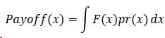
Using this definition, we incorporate any nonlinearities or utility (or values as we tend to call them in SYST 573) of the potential payoffs explicitly using the F(𝑥) function. For decisions with only binary possible payoffs, F(𝑥)=1, so in that case, the payoff function becomes the simple probability of exceeding x, since the final outcome is either 0 or 1, or sometimes −1 or 1, in other words, it becomes 1 − 𝐶𝐷𝐹(𝑥).

Furthermore, using this general model, in order to incorporate more complicated (higher order) potential payoffs, the F(𝑥) can be made more complex to include this. For example, if the payoff of the decision under consideration depends on a simple expectation, i.e., Payoff(x) = E[x], then the corresponding function F(x) = x. It is crucial that we either ignore or don’t overweight frequencies of success or failure or positive or negative outcomes regardless of their magnitude, since it is the total payoff that matters. As Taleb states “One can be right 99% of the time, but this does not matter at all, since with some skewed distributions, the consequences of the expectation of the 1% error can be too large.”

1.2 The Four Quadrant Map

First Quadrant: Simple (binary) decisions, i.e., decisions with simple payoff functions, that are only exposed to Type-1 Randomness. In the first quadrant, the past data used for forecasting doesn’t omit any consequential silent risks, so you may forecast away to your heart’s desire when you are working within it. Unfortunately, however, the majority of difficult real-world decisions under conditions of uncertainty and opacity do not take place in the first quadrant. Several examples of decisions within the first quadrant are: Casino bets, prediction markets, predicting the outcomes of political elections (e.g., what Nate Silver and 538 are famous for).

Second Quadrant: Decisions with complex payoffs which have exposure to Type-1 Randomness/Potential Volatility. Statistical methods may work satisfactorily for decision problems within the second quadrant, though there are still some risks involved here as well. The leftover risks present when you are in the thin-tailed domain are things like the decision-making context you find yourself in does not converge quickly enough to idealized asymptotic properties to justify you using them, that is, you will have to resort to using its preasymptotic properties, lack of independence, and model specification errors. That being said, ways to address these more traditional problems have already been worked out in the literature by statisticians (see Freedman, 2007).

Third Quadrant: Decisions with simple payoff functions which are only exposed to Type-2 Randomness. In this quadrant, there is little risk caused by the predictions you base your decisions on turning out to be wrong because as a result of your decisions being subject to only simple potential payoffs, you are not exposed to the effects of any dramatic, impactful rare events which were not predictable before they happened.

Fourth Quadrant: Decisions with complex payoff functions subject to what Taleb calls Type-2 Randomness in his 4 Quadrant paper and Extremistan in his popular works, and Benoit Mandelbrot called “wild type” randomness. It is in this quadrant that there are truly existential risks caused by decision makers and/or the decision/risk analysts advising them relying on naïve (unnecessarily literal) understandings of the canonical versions of statistical, econometric, and/or machine learning models. We need to avoid relying on forecasts when making decisions with the potential of having remote payoffs altogether, though this is not necessarily true for decisions with simple or more ordinary payoffs. Payoffs from remote parts of any distribution are more difficult to predict than are payoffs from their centers.

1.3 Guidelines for Decision-Making in the Fourth Quadrant

A general principle and guide to practice for decision makers: while making decisions within the first three quadrants, you can safely use the best/optimal analytical model you can fit to the data, it is inadvisable and downright dangerous to do so when the decision at hand takes place in the fourth quadrant. So, the best course of action in practical settings is to exit the fourth quadrant entirely if you can.

What does that mean though? Exiting the fourth quadrant sounds doable, but how does one do this and where do you go from there? The recommendation is to move laterally from the fourth quadrant into the third quadrant.

While it is usually not possible to change the true underlying distribution that describes the context you find your firm or organization in; it is almost always possible to change the payoff function for your decision(s) by changing your exposure(s). This simple heuristic as a guide for when to rely on statistical/analytical models and when to avoid doing entirely is simple to follow in practice.

Plane Crash Analogy

To see the main difference between how one should approach decision making when in the 4th Quadrant, consider the event of a plane crash. A lot of people will lose their lives if almost any given commercial flight crashes, something very sad, say between 100 and 400 people, so the event is counted as a bad episode, but only a single one.

For the sake of forecasting and risk management, we work on minimizing such a probability to make it negligible. Now, imagine, if you would, a type of plane crash that would kill all the people who ever rode on that plane; that is, it will kill all of the people who are riding on it the moment it crashes, and on top of that, all of the passengers who ever rode the plane in the past. All. Should this hypothetical type of plane crash be categorized in the same way as normal plane crashes? The latter event is in Extremistan and, for these, we ought to avoid focusing narrowly and/or naively about probability by itself, but focus instead on the maximum and minimum possible magnitude of the event, should it occur.

(i) When Making Decisions in the Fourth Quadrant, forget about Forecasting Future Outcomes and Focus on the Concavity and Convexity of Your Exposures Instead

As a simple example, say you as the Decision & Risk Analyst, or the Financial Forecasting department of your firm thinks a particular company which is publicly traded has a substantial likelihood of going belly up (going bankrupt) over the next year or two, instead of buying ‘naked’ short positions against that company’s stock price, buy put options against that company’s stock price instead.

What this does is alter your firm’s exposure as opposed to its expected returns. Buying a naked short against some company’s stock price results in your firm having a concave exposure with respect to that short position. Let’s say as an example that the spot price for the stock of the company you are thinking about shorting is $60, the maximum possible return per share of the shorted stock your firm can achieve would be $60, so there is a hard upper bound on the payoff function for this decision, but it the possible losses from this decision are unbounded because that stock could go up to any amount.

If instead of purchasing naked short positions (on N shares) on the company whose stock price you expect to go down over either the short or medium term (or both), you purchase N put options on their stock price, will have reversed you’re the payoff function for your firm’s decision from being concave, that is, one with limited/bounded possible profits and unlimited possible losses) to its opposite, a convex payoff function, that is, limited possible losses and unlimited possible profits. Let’s say that each put option costs $10, then the maximum possible losses for purchasing N put options against this company’s stock price is $10×N.

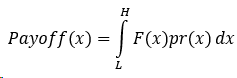
To put the justification for this method for exiting the fourth quadrant more formally (using moments), Taleb states the following in section 7.1 of his aforementioned 4th Quadrant paper (Taleb, 2009):

All moments of the distribution become finite in the absence of open-ended payoffs, by putting a floor 𝐿 below which F(𝑥) = 0, as well a ceiling 𝐻. Just consider that if you are integrating payoffs in a finite, rather than an open-ended domain, i.e. between 𝐿 and 𝐻, respectively, the tails of the distributions outside that domain no longer matter.

(ii) Fragility is a Major Problem, but Antifragility Comes to the Rescue

The concavity of your payoff function for consequences of choosing one decision alternative available to you or your firm is a property of that decision alone, or even more narrowly, that particular alternative for that decision. And while this undesirable property of any particular decision or decision option is important to eliminate in the way described in the previous section, there is also a more general (and thus, much more dangerous) way version of this.

This would be the situation in which your firm as a whole tends to have concave potential payoffs for most or all of its decisions and activities, usually as a result of the industry it is in or the type of services it provides. An example of this would be two common bank types, both nationwide banks which offer standard savings and checking accounts to whoever wants one and also issue or underwrite mortgages to prospective home buyers (assuming they hold on to these mortgages until maturity rather than selling bundles of the mortgages on their balance sheets as “Mortgage Backed Securities” to large investment banks almost immediately after issuing them).

Firms that face concave payoff functions overall or on net balance are fragile (Taleb, 2012). Fragility here means roughly the same things it does when referring to physical objects, for physical objects, for instance, for a cup, fragility means that it can only be damaged or broken by random events it was not designed for such as you accidentally dropping it.

Similarly, the type of banks described above and investment banks as well are much more likely to go bankrupt or “bust” due to a completely unforeseen 20%, 40%, 60%, or larger percentage drop in the market they operate in or in an asset or several assets which dominate their balance sheet in one afternoon, or over a couple of days than they are ever to experience the opposite.

That is to say, large, unexpected events are more likely to damage or bankrupt banks than they are to deliver massive profits, in fact, the latter event has never happened to investment banks, but the former has 3 times in the last 40 years alone (1982, 1987, 2008/2009).

And similarly to how the solutions to the existential threats having concave exposures with respect to the possible consequences of a single decision or a single feasible alternative for a given decision facing your firm is to transform the payoff function resulting from your decision into a convex payoff function in the manner described in the previous section, doing so for your firm or organization overall would be to transform it from a fragile firm into an antifragile firm (Taleb, 2012).

The “Barbell Strategy” is a useful general approach for how to transform yourself or the entity you work for from being fragile to being antifragile which Taleb introduces, explains, and provides several examples of in both his best selling work to date, The Black Swan (Taleb, 2007), and in what in my humble opinion, is clearly his magnum opus, Antifragile (Taleb, 2012), and is referenced in his Fourth Quadrant paper as well (Taleb, 2009). This novel method of risk management and mitigation is outlined in the following sub-section.

(iii) The Barbell Strategy: The Simplest Antifragile Strategy to Implement

The easiest and simplest example of a Barbell Strategy (more technically described as a bimodal strategy) would be an investment portfolio, whether it is a single individual’s portfolio, or that of a large institution or firm he or she works for that they could implement as a way to hedge both unknown and unknowable remote and large left tail events!

A very simple example of a barbell strategy for a regular citizen would be if they were to take all the money currently in their retirement accounts, usually these are a 401k, IRA, or Roth IRA, and put 80–90% of it into a savings account, a money market fund, or treasury bills, something that is completely safe and consequently has an extremely low rate of return.

Then, they put the remaining 10–20% of their retirement nest-egg in a highly speculative, high risk and high reward type of assets, it could be penny stocks, crypto, junk bonds, or something else, but here is the bottom line, in doing this, they have eliminated the maximum possible amount of their retirement fund they could lose to 10 or 20%.

The problem with 401ks and IRAs is that they are presented as being medium risk and in some ways they are year to year, but when 100% of your retirement fund is in such accounts which means that it is actually in some mixture of stocks and bonds, you are exposed a maximum possible loss of 100% of your retirement fund.

1.5 Related Issue of the Conflation of Events and Exposures

x vs f(x), exposures to x confused with knowledge about x

The material in this sub section comes from the Chapter 3, section 9 of Nassim Taleb’s 2020 monograph The Technical Inceto (Volume 1): Statistical Consequences of Fat Tails: Real World Preasymptotics, Epistemology, and Applications.[4]

This is actually more than just a “related” issue, this is more or less a different way to frame the same issue, the same vital distinction that I just covered throughout parts 1.1-1.4, which is different, and more concise. So, if you did not follow all of that, here’s another way to think about it.

Once again, like in section 1.3, let’s say x is a random or nonrandom variable that represents the outcome of an event, and F(x) is the exposure or payoff, i.e., the effect of x on you. In order to simplify things, we will assume that x is only a simple, one-dimensional variable, but in reality, it can of course be of a higher dimensional.

Practitioners (decision makers), real-world doers, and risk takers often observe the following disconnect: nonpractitioners talking a lot about x, some future event (with the implication that these nonpractitioners assume that practitioners do or should care about x when making decisions), but they are completely off the mark, practitioners only care about F(X), the exposure to the consequences of that event, should it happen, and nothing but F(X)!

According to Taleb, when it comes to probability theory, the more nonlinear the payoff function F(x) is, the less the probability of the event x happening matter compared to that of F(x). Moral of the story: focus on your exposure or payoff from events, which you can typically alter more directly, rather than on the measurement of the elusive properties of unknown possible events that may happen.

Fragility and Antifragility

When your exposure to an event is concave, you are Fragile with respect to that event, errors in your prediction about the event itself can translate into extreme negative values for your payoff. When your exposure is convex, you are largely immune from severe negative variations.

In situations of trial and error, or with an option, we do not need to understand events or how likely they are to happen as much as we need to understand our exposure to the risks of their potential consequences. Simply put, the statistical properties of x are totally swamped by those of H. The H in the payoff function from section 1.3:

The thesis of Taleb’s magnum opus, Antifragile, is that exposure is much more important than the naive notion of, “knowledge”, that is, understanding x or thinking you can accurately predict it. The more nonlinear the payoff F(x) is, the less the probability of x matters than the probability distribution of the payoff. Many people confuse the probabilities of x with those of F(x), including the authors of the textbook used for this course occasionally.

A part II article on Preasymptotics, the Law of Medium Numbers, and the Law of Averages can be found here.

References

[1] Freedman, D. (2007). Statistics (4th edition). W.W. Norton & Company.

[2] Kirkwood, C. W. (2020). Strategic Decision Making: Multiobjective Decision Analysis with Spreadsheets. Wadsworth Publishing Company.

[3] Taleb, N. N. (2012). Antifragile: things that gain from disorder. Random House.

[4] Taleb, N. N. (2009). Errors, Robustness, and The Fourth Quadrant. International Journal of Forecasting, 25(4), 744–759. https://www.sciencedirect.com/science/article/abs/pii/S016920700900096X

[5] Taleb, N. N. (2020). Statistical Consequences of Fat Tails: Real World Preasymptotics, Epistemology, and Applications. STEM Academic Press. https://arxiv.org/abs/2001.10488

[6] Taleb, N. N. (2007). The Black Swan: the impact of the highly improbable. US: Random House.

[7] Taleb, N. N. (2008). The Fourth Quadrant: A Map of The Limits of Statistics. From Edge.org. https://www.edge.org/conversation/nassim_nicholas_taleb-the-fourth-quadrant-a-map-of-the-limits-of-statistics