
Blindspots in the Standard Risk and Decision Theory Curriculum
I Took a Graduate Level Course on Decision & Risk Analysis and it was Painfully Out of Date, Here are Some Considerations I Would Update the Material With
Note: I was told I could do a solo final paper for the class after missing the deadline to join a team for a group project due to a temporary health emergency, and after being alarmed at how out of date some of the material still was given my knowledge and admiration of the work in Risk and Decision Theory by the loveably cantankerous Nassim Nicholas Taleb, so I asked my professor if I could write a long paper explaining the updates to the curriculum of the course itself I strongly feel should be made and he was intrigued enough by my moxy in asking him to do so that he agreed. This is that paper.
Overview & Motivation
This research report for SYST 573 — Decision and Risk Analysis (at George Mason Univserity) presents underappreciated problems that arise when real world risk analysts and decision makers commit the error of relying too heavily on idealized versions of standard statistical, machine learning, or econometric modeling and forecasting techniques without understanding when these methods of analysis work the way academic textbooks claim they work (in Large samples or Asymptotically, but fail to provide any guidance whatsoever on how to know where your sample is large enough across all possible types of underlying probability distributions).
It then goes on the provide alternative heuristics and decision-making guidelines you can rely on when you don’t know if your sample or source data is large enough to justify direct application of classical elementary notions of statistical inference in the decision-making context you are faced with.
After that, analytical justifications and graphical explanations are provided to demonstrate exactly why most sophisticated analytical modeling and forecasting methods are valid much less often than most people, including applied statisticians and data scientists realize. This error has been identified in the literature as The Law of Medium Numbers, and the final part of this report highlights its relationship with the already well understood error known as The Law of Averages.
Part 1: Nassim Taleb’s Four Quadrant Model — A Map of the Practical Limitations of Statistics in the Real World
1.1 Introduction, Motivation, and Purpose of this Article
Most of the new concepts, categories, and decision making guidelines discussed in Part 1 of this report comes from the peer-reviews journal article, Nassim Taleb’s landmark 2009 paper “Errors, Robustness, and the Fourth Quadrant,” which was written by the maverick probabilist, former options and financial derivatives trader, risk taking theorist, and fragility/antifragility theory pioneer, Dr. Nassim Taleb (who has been a quarter time Distinguished Professor of Risk Engineering at the NYU’s Tandon School of Engineering since September 2008 when he retired from his long career as an options trader), and published in 2009 in the International Journal of Forecasting.
I’ll start off with a quote from the paper itself: “The extensive literature on decision theory and choices under uncertainty so far has limited itself to (1) assuming known probability distributions (except for a few exceptions in which this type of uncertainty has been called “ambiguity”, and (2) ignoring fat tails. This paper introduces a new structure of fat tails and classification of classes of randomness into the analysis and focuses on the interrelation between errors and decisions.”
The new framework introduced in the paper partitions types of decisions along with their corresponding exposures to unforeseen (and often unforeseeable) risks into four different categories, or “Quadrants,” by dividing them into two qualitatively and quantitively distinct types of decisions in terms of the possible payoffs which result as a consequence of those decisions along two different dimensions (qualitatively different levels of randomness), leading to a total of four mutually exclusive and collectively exhaustive “quadrants.”
(i) The Two Types of Decisions
The first type of decisions are simple decisions with only binary potential payoffs. For these simple decisions with binary payoffs, the only matter of concern is whether your belief, claim, or prediction is True or False, there is no such thing something being “very true” or “extremely false.” So, for instance, if you are a fertility doctor seeing a female patient who wants to know the results of a pregnancy test you had her take recently, the only possible results of that pregnancy test are Positive, indicating that she is pregnant, or Negative, indicating that she is not pregnant, she can’t be “very pregnant” or “very not pregnant.”
For these types of decisions, all that matters is the probability that the events will happen, not on their magnitude.1 While very easy to deal with, unfortunately, this type of decision is not very common in everyday life either as a common citizen in personal matters or as a Decision Maker or Stakeholder at a firm. A few examples of this type would be placing a bet on the outcome of a democratic election or a fixed bet on the outcome of someone flipping a (fair) coin, or perhaps laboratory experiments of hypotheses by researchers.
The second type of decisions are those subject to complex potential payoffs. The Decision Maker does not (or at least, he need not) care about how frequently the predictions on which he bases his decisions are accurate, but about the impact or magnitude of the payoffs, and the cumulative effect of the interaction between the overall accuracy rate of the predictions made during the process of making many decisions over time multiplied by the magnitude of the payoffs received or penalties incurred as their consequences.
These payoffs depend on higher moments of the underlying distributions. Put more simply, when one invests, he cares not about the frequency of the momentary increases or decreases in the value of that investment; instead, he cares about their overall expectation, i.e., how many times the value increased or decreased multiplied by the corresponding magnitudes of each of those increases and decreases. In extreme cases of type 2 decisions, as Taleb puts it:
“One can be right 99% of the time, but this does not matter at all, since with some skewed distributions, the consequences of the expectation of the 1% error can be too large.”
(ii) The Two Probabilistic Domains
Most statisticians, whether applied or theoretical, when they divide up different probability distributions into groups of related distributions, they do so in terms of what refer to as families of probability distributions (e.g. the Gamma family, Exponential family, Gaussian family, etc.). However, the motivation behind these categorization schemes are purely mathematical considerations, such relationships between distributions in terms of having shared shape or location parameters and the like, but these families are not very practically useful for Decision Analysts or Decision Makers.
That crucial practical gap was Taleb’s fundamental purpose for his Four Quadrants paper. His novel categorization scheme for probability distributions intended for practical purposes by Decision Makers, not Ivory Tower professors who never decide anything important, divides all of them into one of just two different domains. These two domains are quite distinct qualitatively, quantitatively, and practically.
The first probabilistic domain is the class of all probability distributions subject to what he calls Type-1 Randomness, which includes all probability distributions which are “benign” in terms of their kurtosis. A particular probability distribution which has only a mesokurtic shape profile, that is, its overall kurtosis is close to 3, therefore, its excess kurtosis is close to 0. they have thin-tails and are nonscalable. In his popular books, Taleb refers to this probabilistic domain as Mediocristan.
The second probabilistic domain includes all probability distributions subject to what he calls Type-2 Randomness. The second domain is that which is includes all probability distributions which are significantly leptokurtic, i.e., they have thick-tails or a long-tail (often referred to informally as “fat-tails”) and are scalable (or even fractal). In his popular books, Taleb refers to this probabilistic domain as Extremistan.
To restate the above distinctions in a more formal manner, let us denote the probability distribution of some random variable 𝑥 as 𝑝𝑟(𝑥), and 𝐷 as the domain over which this probability distribution is defined, then its payoff function is defined as:
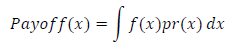
Using this definition, we incorporate any nonlinearities or utility (or values as we tend to call them in SYST 573) of the potential payoffs explicitly using the 𝑓(𝑥) function. For decisions with only binary possible payoffs, 𝑓(𝑥)=1, so in that case, the payoff function becomes the simple probability of exceeding x, since the final outcome is either 0 or 1, or sometimes −1 or 1, in other words, it becomes 1 − 𝐶𝐷𝐹(𝑥). Furthermore, using this general model, in order to incorporate more complicated (higher order) potential payoffs, the 𝑓(𝑥) can be made more complex to include this.
1.2 The Map
First Quadrant: Simple (binary) decisions, i.e., decisions with simple payoff functions, that are only exposed to Type-1 Randomness. In the first quadrant, the past data used for forecasting doesn’t omit any consequential silent risks, so you may forecast away to your heart’s desire when you are working within it. Unfortunately, however, the majority of difficult real-world decisions under conditions of uncertainty and opacity do not take place in the first quadrant. Several examples of decisions within the first quadrant are: Casino bets, prediction markets, predicting the outcomes of political elections (e.g., what Nate Silver and 538 are famous for).
Second Quadrant: Decisions with complex payoffs which have exposure to Type-1 Randomness/Potential Volatility. Statistical methods may work satisfactorily for decision problems within the second quadrant, though there are still some risks involved here as well. The leftover risks present when you are in the thin-tailed domain are things like the decision-making context you find yourself in does not converge quickly enough to idealized asymptotic properties to justify you using them, that is, you will have to resort to using its preasymptotic properties, lack of independence, and model specification errors. That being said, ways to address these more traditional problems have already been worked out in the literature by statisticians (see Freedman, 2007).
Third Quadrant: Decisions with simple payoff functions which are only exposed to Type-2 Randomness. In this quadrant, there is little risk caused by the predictions you base your decisions on turning out to be wrong because as a result of your decisions being subject to only simple potential payoffs, you are not exposed to the effects of any dramatic, impactful rare events which were not predictable before they happened.
Fourth Quadrant: Decisions with complex payoff functions subject to what Taleb calls Type-2 Randomness and Benoit Mandelbrot called “wild type” randomness. It is in this quadrant that there are truly existential risks caused by decision makers and/or the decision/risk analysts advising them relying on naïve (unnecessarily literal) understandings of the canonical versions of statistical, econometric, and/or machine learning models. We need to avoid relying on forecasts when making decisions with the potential of having remote payoffs altogether, though this is not necessarily true for decisions with simple or more ordinary payoffs. Payoffs from remote parts of any distribution are more difficult to predict than are payoffs from their centers.
1.3 Guidelines for Decision-Making in the Fourth Quadrant
A general principle and guide to practice for decision makers: while making decisions within the first three quadrants, you can safely use the best/optimal analytical model you can fit to the data, it is inadvisable and downright dangerous to do so when the decision at hand takes place in the fourth quadrant. So, the best course of action in practical settings is to exit the fourth quadrant entirely if you can.
What does that mean though? Exiting the fourth quadrant sounds doable, but how does one do this and where do you go from there? The recommendation is to move laterally from the fourth quadrant into the third quadrant.
While it is usually not possible to change the true underlying distribution that describes the context you find your firm or organization in; it is almost always possible to change the payoff function for your decision(s) by changing your exposure(s). This simple heuristic as a guide for when to rely on statistical/analytical models and when to avoid doing entirely is simple to follow in practice.
(i) When Making Decisions in the Fourth Quadrant, forget about Forecasting Future Outcomes and Focus on the Concavity and Convexity of Your Exposures Instead
As a simple example, say you as the Decision & Risk Analyst, or the Financial Forecasting department of your firm thinks a particular company which is publicly traded has a substantial likelihood of going belly up (going bankrupt) over the next year or two, instead of buying ‘naked’ short positions against that company’s stock price, buy put options against that company’s stock price instead.
What this does is alter your firm’s exposure as opposed to its expected returns. Buying a naked short against some company’s stock price results in your firm having a concave exposure with respect to that short position. Let’s say as an example that the spot price for the stock of the company you are thinking about shorting is $60, the maximum possible return per share of the shorted stock your firm can achieve would be $60, so there is a hard upper bound on the payoff function for this decision, but it the possible losses from this decision are unbounded because that stock could go up to any amount.
If instead of purchasing naked short positions (on N shares) on the company whose stock price you expect to go down over either the short or medium term (or both), you purchase N put options on their stock price, will have reversed you’re the payoff function for your firm’s decision from being concave, that is, one with limited/bounded possible profits and unlimited possible losses) to its opposite, a convex payoff function, that is, limited possible losses and unlimited possible profits. Let’s say that each put option costs $10, then the maximum possible losses for purchasing N put options against this company’s stock price is $10×N.
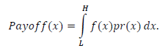
To put the justification for this method for exiting the fourth quadrant more formally (using moments), Taleb states the following in section 7.1 of his aforementioned 4th Quadrant paper (Taleb, 2009):
All moments of the distribution become finite in the absence of open-ended payoffs, by putting a floor 𝐿 below which 𝑓(𝑥) = 0, as well a ceiling 𝐻. Just consider that if you are integrating payoffs in a finite, rather than an open-ended domain, i.e. between 𝐿 and 𝐻, respectively, the tails of the distributions outside that domain no longer matter.
(ii) Fragility is a Major Problem, but Antifragility Comes to the Rescue
The concavity of your payoff function for consequences of choosing one decision alternative available to you or your firm is a property of that decision alone, or even more narrowly, that particular alternative for that decision. And while this undesirable property of any particular decision or decision option is important to eliminate in the way described in the previous section, there is also a more general (and thus, much more dangerous) way version of this.
This would be the situation in which your firm as a whole tends to have concave potential payoffs for most or all of its decisions and activities, usually as a result of the industry it is in or the type of services it provides. An example of this would be two common bank types, both nationwide banks which offer standard savings and checking accounts to whoever wants one and also issue or underwrite mortgages to prospective home buyers (assuming they hold on to these mortgages until maturity rather than selling bundles of the mortgages on their balance sheets as “Mortgage Backed Securities” to large investment banks almost immediately after issuing them).
Firms that face concave payoff functions overall or on net balance are fragile (Taleb, 2012). Fragility here means roughly the same things it does when referring to physical objects, for physical objects, for instance, for a cup, fragility means that it can only be damaged or broken by random events it was not designed for such as you accidentally dropping it.
Similarly, the type of banks described above and investment banks as well are much more likely to go bankrupt or “bust” due to a completely unforeseen 20%, 40%, 60%, or larger percentage drop in the market they operate in or in an asset or several assets which dominate their balance sheet in one afternoon, or over a couple of days than they are ever to experience the opposite.
That is to say, large, unexpected events are more likely to damage or bankrupt banks than they are to deliver massive profits, in fact, the latter event has never happened to investment banks, but the former has 3 times in the last 40 years alone (1982, 1987, 2008/2009).
And similarly to how the solutions to the existential threats having concave exposures with respect to the possible consequences of a single decision or a single feasible alternative for a given decision facing your firm is to transform the payoff function resulting from your decision into a convex payoff function in the manner described in the previous section, doing so for your firm or organization overall would be to transform it from a fragile firm into an antifragile firm (Taleb, 2012).
The “Barbell Strategy” is a useful general approach for how to transform yourself or the entity you work for from being fragile to being antifragile which Taleb introduces, explains, and provides several examples of in both his best selling work to date, The Black Swan (Taleb, 2007), and in what in my humble opinion, is clearly his magnum opus, Antifragile (Taleb, 2012), and is referenced in his Fourth Quadrant paper as well (Taleb, 2009). This novel method of risk management and mitigation is outlined in the following sub-section.
(iii) The Barbell Strategy: The Simplest Antifragile Strategy to Implement
The easiest and simplest example of a Barbell Strategy (more technically described as a bimodal strategy) would be an investment portfolio, whether it is a single individual’s portfolio, or that of a large institution or firm he or she works for that they could implement as a way to hedge both unknown and unknowable remote and large left tail events!
A very simple example of a barbell strategy for a regular citizen would be if they were to take all the money currently in their retirement accounts, usually these are a 401k, IRA, or Roth IRA, and put 80–90% of it into a savings account, a money market fund, or treasury bills, something that is completely safe and consequently has an extremely low rate of return.
Then, they put the remaining 10–20% of their retirement nest-egg in a highly speculative, high risk and high reward type of assets, it could be penny stocks, crypto, junk bonds, or something else, but here is the bottom line, in doing this, they have eliminated the maximum possible amount of their retirement fund they could lose to 10 or 20%.
The problem with 401ks and IRAs is that they are presented as being medium risk and in some ways they are year to year, but when 100% of your retirement fund is in such accounts which means that it is actually in some mixture of stocks and bonds, you are exposed a maximum possible loss of 100% of your retirement fund.
Part 2: The Law of Medium Numbers
The Law of Large Numbers, The Central Limit Theorem, Rates of Convergence Towards the LLN & CLT for Different Distributions, and Preasymptotics
2.1 Introduction and Purpose of Part 2
Everything presented in Part 2 of this report comes from either chapters 7 and 8 of Taleb’s 2020 monograph Statistical Consequences of Fat Tails: Real World Preasymptotics, Epistemology, and Applications.
The preasymptotic properties of the probability distributions which accurately characterize the population, phenomenon, or process within which important decisions take place are the only properties that ought to be considered by Decision Makers, Stakeholders, and the Decision and/or Risk Analysts tasked with aiding them in making these decisions when the rate of convergence towards the Gaussian Distribution for the true underlying distributions is (sufficiently) slow.
Whether you are a Decision Maker or a Decision and/or Risk Analyst advising a Decision Maker in a firm the private sector, a nonprofit organization, a government department, or even a general in the armed forces, naively relying on theories which were derived in idealized situations, such as properties which only occur asymptotically, can be extremely dangerous in practice. Using the wrong model can often be worse than not using any formal models at all to guide you.
2.2 The Law of Large Numbers
In plain English, The Law of Large Numbers tells you that as more and more additional observations are added to your sample, the mean of your sample becomes more and more stable. That is, as the size of your sample, n, grows, it its mean, i.e., your sample mean, becomes a better and better estimate of the true underlying (and unobservable) population mean.
The gist/take-home message of both the weak and strong version of the LLN is this: For all sets of 𝑛 random variables, that is, {𝑋1,𝑋2,𝑋3,…,𝑋𝑛}, the sample mean, i.e.,
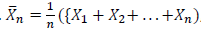
, converges to the population mean, i.e., the Expected Value, 𝑋𝑛 → 𝜇, as 𝑛 → ∞.
(i) The Weak & Strong Versions of The Law of Large Numbers
The Weak LLN: The weak law of large numbers can be summarized as follows: the probability of a variation in excess of some threshold for the average becomes progressively smaller as the sequence progresses. In estimation theory and econometrics, an estimator is called consistent if it thus converges in probability to the quantity being estimated (aka, the “estimand”):

when 𝑛 → ∞. Or, if you prefer the epsilon-delta definition of limits, then the Weak LLN can be expressed as:

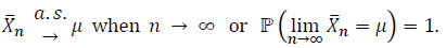
The Strong LLN: The Strong Law of Large Numbers states that, as the number of sample summands, 𝑛, goes to infinity, the probability that the average of those sample summands converges to the population average (Expected Value) is equal to 1 asymptotically. This can be expressed as:
Both versions of the LLN are great, they make teaching statistics courses easier because the professor can just pretend everything is described by a Gaussian due to the LLN, but there is an important consideration which he and the rest of his profession must consider, but had not before Taleb came along (according to Taleb, “The “speed” (of convergence), appears to have been ignored (by the statistics community), there is almost no mention of it among the 9,400 pages of the Encyclopedia of Statistical Science.”)
That consideration is how quickly the distribution which accurately characterizes the probabilistic domain in which they are operating converges, via The Law of Large Numbers, to having sufficiently similar properties and characteristics as the Gaussian in order to safely substitute it for the real underlying Distribution.
That is, they ought first to consider the rate or “speed” of the convergence towards the Gaussian via the operation of the LLN (just how “large” does our sample need to be) in comparison to the number of observations, i.e. the sample size, they actually have available to them.
2.3 The Central Limit Theorem
According to the introductory article on the Central Limit Theorem on Statistics How To website (Glen, 2022):
“The Central Limit Theorem states that the sampling distribution of the sample means approaches a normal distribution as the sample size gets larger — no matter what the shape of the (true underlying) population distribution is.”
All this is saying is that as you draw more and more samples, especially large ones, the histogram of the distribution of your sample means, i.e. the graph of their sampling distribution, will look more and more like the graph of an idealized normal distribution (the familiar “bell curve”).
Graphically Exploring Monte Carlo Simulations to Show the 4 Qualitatively Distinct Operational Rates of Convergence to the Gaussian via the LLN and/or the CLT in Practice for Various Types of Underlying Probability Distributions
We note that if X has a finite variance, the stable-distributed random variable X_s will be Gaussian. But note that X_s is a limiting construct as n → ∞ and there are many, many complication with “how fast” we get there. Let us consider 4 cases that illustrate both the idea of CLT and the speed of it.
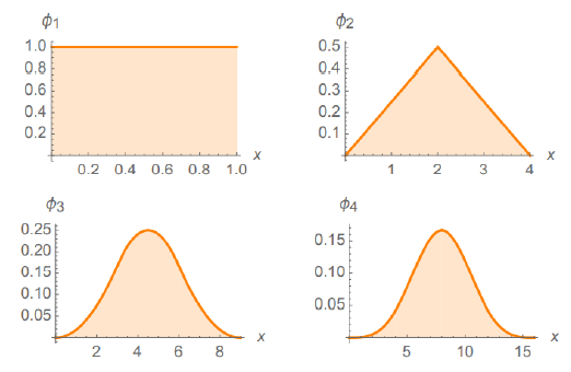
- Fastest Convergence: The Uniform Distribution.
The extremely fast rate of convergence to the Gaussian when summing a set of 2 or more Uniformly Distributed random variables can be seen in Figure 1. Summing together just 2 i.i.d Uniform Random Variables results in the Triangular Distribution.
The Stable Distributions
Using the same notation as above, let X_1, . . . , X_n be independent and identically distributed random variables. Consider their sum Sn. We have
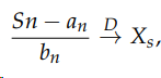
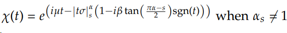
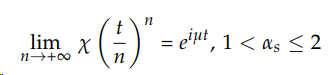
where X_s follows a stable distribution S, a and bn are norming constants, and, to repeat, → (with a D above it) denotes convergence in distribution (the distribution of X as n → ∞). The properties of S will be more properly defined and explored in the next chapter. Take it for now that a random variable Xs follows a stable (or α-stable) distribution, symbolically Xs ∼ S(α_s, β, µ, σ), if its characteristic function χ(t) = E(e^itX_s) is of the form:
The constraints are −1 ≤ β ≤ 1 and 0 < α_s ≤ 2.
The designation stable distribution implies that the distribution (or class) is stable under summation: you sum up random variables following any the various distributions that are members of the class S explained next chapter (actually the same distribution with different parametrizations of the characteristic function), and you stay within the same distribution.
Intuitively, χ(t)^n is the same form as χ(t) , with µ → nµ, and σ → n^(1/α)σ. The well known distributions in the class (or some people call it a “basin”) are: the Gaussian, the Cauchy and the Lévy with α = 2, 1, and 1 2 , respectively. Other distributions have no closed form density.
The Law of Large Numbers for the Stable Distribution
Let us return to the law of large numbers.
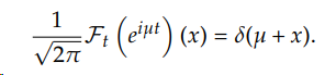
By standard results, we can observe the law of large numbers at work for the stable distribution, as illustrated in Figure 2:
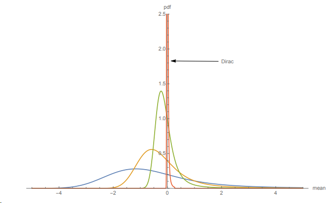
which is the characteristic function of a Dirac delta at µ, a degenerate distribution, since the Fourier transform F (here parametrized to be the inverse of the characteristic function) is:
Further, we can observe the “real-time” operation for all 1 < n < +∞ in the following ways, as we will explore in the next sections.
2. Semi-Slow Convergence: The Exponential Distribution.
A sum of Exponential Random Variables converges to the Gaussian somewhat more slowly than a sum of Uniform Random Variables mostly on account of the skewness of The Exponential Distribution, but still quickly enough to justify substituting the Gaussian for the Exponential in your analysis or modeling without potentially catastrophic consequences of doing so.
The initial probability density function is:
and for n summands, it is:
You can see how we get more slowly to the Gaussian, as shown in Figure 2, mostly on account of its skewness. Getting all the way to the Gaussian Distribution requires symmetry.
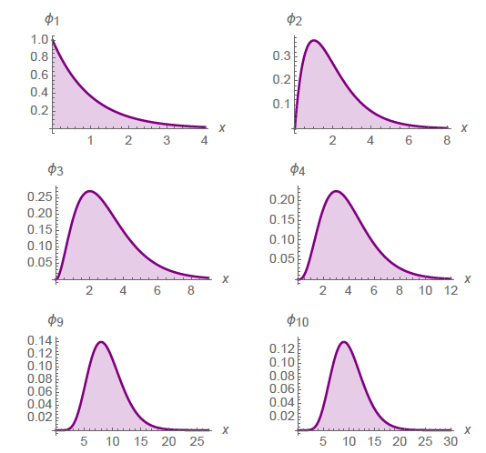
3. Slow Convergence: The slow Pareto Distribution.
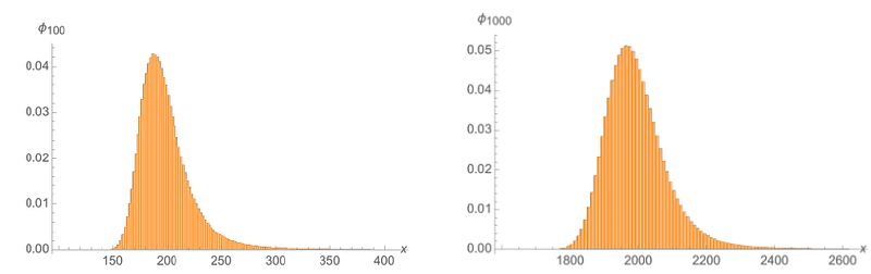
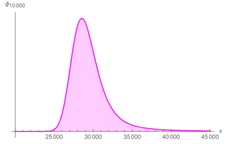
Because the simplest versions of the Pareto Distribution are the “greyest” (that is, least “black & white” of the 4 different convergence speeds presented here), I include two figures, one with 9 individual graphs showing the resulting joint distributions when summing up 1–9 Pareto Random Variables and another showing how the same for join distributions resulting from summing up 100 & 100 Pareto R.V.s in order to show just how slow the convergence here really is.
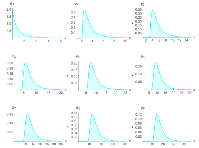
Consider the simplest Pareto distribution on [1, ∞):
and inverting the characteristic function,
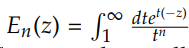
Where E(.) (.) is the exponential integral
Clearly, the integration is done numerically (so far nobody has managed to pull out the distribution of a Pareto sum). It can be exponentially slow (up to 24 hours for n = 50 vs. 45 seconds for n = 2), so we have used Monte Carlo simulations to create Figure 2.
4. Glacially Slow Convergence: The half-cubic Pareto Distribution never becomes symmetric in real life.
The bottom line when it comes to the slowness of the convergence to stable, Pareto Distributed final values of Pareto Distributions in practice towards Gaussian properties via the LLN and/or the CLT in practical applications being much too slow to warrant substituting the Gaussian for analysis, forecasting, or modeling when you may be operating in a fat-tailed domain is made even clearer in the table 1 below.
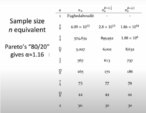
In table 1, the top sample minimum sample size number in the first row, Fuhgeddaboudit is a sarcastic way of saying “Forget about it” because you are never going to get there with real world source datasets.
To summarize the most salient information in Table 1, as opposed to the Gaussian, for which you can draw valid statistical inferences with a minimum necessary sample size of only 30 (a Pareto with an alpha parameter of 𝛼 = 2 is a Gaussian), depending on the alpha exponent of the Pareto Distribution, it can be anywhere up to trillions or more as the minimum necessary sample size!
2.4 Relationship Between The Law of Medium Numbers and The So-Called The Law of Averages
I am going to be completely honest here, I had never really heard the term “The Law of Averages” until about halfway through writing this report, but apparently, according to roughly the first 3 to 5 results on it I was able to find using both Google search and Bing search, both The Law of Averages in general, and a special case of it known as Gambler’s Fallacy, are quite common among statistically ignorant citizens.
This error is fundamentally a misunderstanding of when the implications of The Law of Large Numbers may be invoked and when they may not be. The hint for when you may invoke the LLN is right there in its name, you need a large number of observations in order to invoke the LLN as a justification for using the easier to work with asymptotic properties of distributions.
As Stephanie Glen puts it, the difference between The Law of Large Numbers and The Law of Averages is the following:
“The Law of Large Numbers states that if you take an unpredictable experiment and repeat it enough times (i.e. for a very big number), what you’ll end up with is an average (expected value); while The Law of Averages is the belief that The Law of Large Numbers also applies to small numbers as well (Glen, 2021).”
The Gambler’s Fallacy occurs when a gambler who has been observing the results of, let’s say, 5 or 10 spins of a roulette wheel, where all of them came up on black, and as a result, he decides to place a substantial bet on the next spin of the wheel as coming up on red because he feels that the universe is “due” for a red spin, and not only that, it is due for a similar streak of reds in a row in order to return the observed sample of spins to its long run average of 50/50 for red and black. The probability of the next spin of the roulette wheel coming up on red is 0.5, the same as it has been for every previous spin and the same as it will be for all subsequent spins.
Hopefully, I have explained everything regarding the two types or domains of randomness back in Part 1, rates of convergence in Part 2, and also The Law of Averages above well enough that the parallels are clear between the error laypersons are making when they mentally substitute The Law of Averages for The Law of Large Numbers and the error analysts are making when they rely on the combination of the LLN & the CLT to be sufficient as justification for them to use the Gaussian Distribution as a default when they don’t know what the true underlying distribution is.
In fact, referring to the relationship between these errors as a “parallel” does not do it justice. If you step back, this is, in fact, the exact same error, they are invoking the right to use the simplifications justified by the LLN and CLT before they have enough sample observations to do so.
References
[1] Freedman, D. (2007). Statistics (4th ed.). W.W. Norton & Company.
[2] Glen, S. (2021). “Law of Large Numbers / Law of Averages” From StatisticsHowTo.com: Elementary Statistics for the rest of us! https://www.statisticshowto.com/law-large-numbers/
[3] Glen, S. (2022). “Central Limit Theorem: Definition and Examples” From StatisticsHowTo.com: Elementary Statistics for the rest of us! https://www.statisticshowto.com/probability-and-statistics/normal-distributions/central-limit-theorem-definition-examples/
[4] Taleb, N. N. (2009). Errors, Robustness, and The Fourth Quadrant. International Journal of Forecasting, 25(4), 744–759. https://www.sciencedirect.com/science/article/abs/pii/S016920700900096X
[5] Taleb, N. N. (2012). Antifragile: things that gain from disorder. Random House.
[6] Taleb, N. N. (2020). Statistical Consequences of Fat Tails: Real World Preasymptotics, Epistemology, and Applications. STEM Academic Press. https://arxiv.org/abs/2001.10488
[7] Taleb, N. N. (2007). The Black Swan: the impact of the highly improbable. US: Random House.
[8] Taleb, N. N. (2008). The Fourth Quadrant: A Map of The Limits of Statistics. From Edge.org. https://www.edge.org/conversation/nassim_nicholas_taleb-the-fourth-quadrant-a-map-of-the-limits-of-statistics


