Introduction to Data Structures and Algorithm — Asymptotic Analysis and the Big O Notation.

Unraveling Data Structures and Algorithms (Part 3): Asymptotic Analysis and the Big O Notation.

Here is what you need to know to get started in Data structures and Algorithms.

Learning Objectives.

Understanding the Growth Rate of Functions.

Exploring the Concept of Big O Notation.

This article is the third in a series that introduces Data Structures and Algorithms. You can find the previous articles here.

Introduction

In the previous chapter, we looked at complexity analysis and how we can analyze an algorithm by counting the number of operations. Now that you’ve learned how we analyze running time. Let us extend that understanding a bit further. We will touch on some key crucial terms like asymptotic analysis and growth rate. This will ensure that you fully grasp the concept of Big O Notation

Growth Rates

A problem could be solved by employing various algorithmic solutions, and computer scientists are tasked with determining the most efficient one. This can be achieved by estimating the growth rate of an algorithm’s running time.

Because the efficiency of some algorithms depends on the input size, scientists have developed ways to categorize algorithms using mathematical notations that ignore constant (non-changing) factors.

There are different growth rates for the running time of an algorithm with respect to any input of size n, as we saw in the previous chapter. We can summarize these growth rates in the table below.

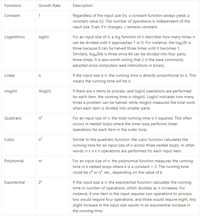
Different functions, growth rate, and their description

As an illustration, If you compare two algorithms — one linear and the other logarithmic — that execute some operations on a specific input n, the difference in running time between the two algorithms may be insignificant if the input has a minimal size, but as the size of the input approaches a vast number, the algorithm with logarithmic running time becomes generally more efficient. We can also say that as the size of the input increases, the linear algorithm grows faster than the logarithmic algorithm.

The Image below demonstrates the growth rate in increasing order for the functions described above.

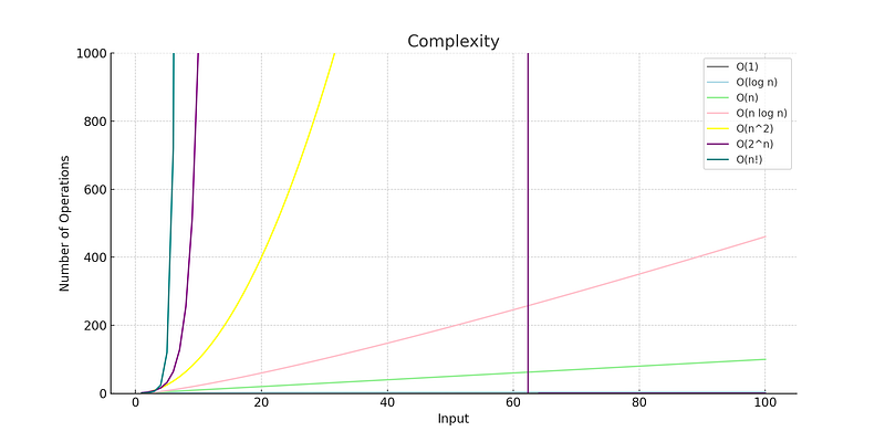
The design process for any algorithm should aim for a minimal number of operations to solve problems. Typically, if the running time of an algorithm is between cubic and exponential, it may be necessary to revisit the design.

Asymptotic Analysis and the Big O Notation,

Think of Big “O” as a way to describe how fast functions grow (running time) as their input size grows. When we say a function is big “oh” of n, i.e., f(n) = O(n), this implies that for any input of size n, the growth rate (running time) is proportional to n. As n increases in size, the running time increases proportionately. On the other hand, f(n) = O(n²) implies that as n increases, the running time increases quadratically (By a factor of two).

Big O also describes the ordering of the properties of a function. For example, the running time of a function expressed as

3n⁴ + 4n³ + 5n² + 6n + 7

is O(n⁴) because as the input size n becomes very large, n⁴ becomes larger than n³ and n² and so on. This means the running time of this function grows by a polynomial order of n⁴, and n⁴ defines the asymptotic running time of this function, ignoring the lower-order polynomials like n³ and constants like 7.

We employ the Big O notation when analyzing running time and space bounds because it abstracts less significant factors and focuses more on the dominant ones.

Big O is also mathematically denoted as:

f(n) ≤ cg(n), for n ≥ n0,

Where c is a constant, representing the sum of the co-efficient of n. c is a real number (positive) greater than 1, like the sum of the numbers 3, 4, 5, 6, and 7 from the example function above. We can represent it as:

3n⁴ + 4n³ + 5n² + 6n + 7 ≤ (3+4+5+6+7).n⁴, for n ≥ n0

which gives us,

3n⁴ + 4n³ + 5n² + 6n + 7 ≤ 25.n⁴, for n ≥ n0

n ≥ n0 means what we have already discussed. As input increases, the running time of certain algorithms becomes more efficient. After a certain input size n0, which could be equal to 1, f(n) (3n⁴ in this case) becomes less than or equal to c.g(n). In our example, 3n⁴ ≤ 25n⁴

f(n) ≤ c.g(n) or, as we generally say, f(n) is O(g(n)) where f(n) and g(n) are two non-negative functions, and c is independent of n meaning it does not change regardless any change in input size n.

Here is another scenario. f(n) can be a function like our BUBBLESORTalgorithm above 3n² - 3n + 3, and g(n) would be n². Hence, the function f(n) is O(n²).

Mathematically, 3n² — 3n + 3 ≤ 3.n² for n ≥ n0.

To prove this, let's substitute some values for n in the equation

At n = 1,

3.1 ² — 3.1 + 3 ≤ 3.1 ² ⇒

3–3 + 3 ≤ 3 ⇒

3 ≤ 3

At n = 2

3.2 ² — 3.2 + 3 ≤ 3.2 ² =>

12–6 + 3 ≤ 12 =>

9 ≤ 12

This shows that for the running time of the bubble sort algorithm 3n² — 3n + 3 ≤ 3.n², fn is O(n²).

The Big O notation analysis is typically categorized into three scenarios.

Worst Case or Big O

Best Case or Big Omega Ω and,

Average Case or Big Theta Θ

Worst Case (Big O) describes the upper bound of the algorithm’s running time, meaning we generally look at the longest amount of time (worst case) an algorithm can possibly take to execute.

Best Case (Big Omega Ω) is the opposite. It looks at the lower bound of an algorithm’s running time, indicating the minimum time it requires to execute.

Average Case (Big Theta Θ) actually describes a tight bound, meaning the algorithm’s running time is both upper-bounded and lower-bounded by the same function representing the average time it takes to complete an algorithm.

Just like in most real-life situations, when dealing with problems, we consider the worst-case scenario. In computer science, we typically focus on the same. Asymptotic Analysis assumes the worst-case scenario or upper bounds of a function. Let me describe an illustration that helped me distinguish these scenarios.

Imagine a race at the Olympics where each country has three members representing them. During the race, members of all the teams will compete at the same time. The winner of the race will be determined by the time it takes for the last person (worst case) to reach the finish line.

Consider there is a US team competing. It does not matter if the first three runners finish under 5 seconds. If the last runner finishes in 20 seconds (worst-case), then the time recorded for the US team will be 20 seconds. The time the other runners took to reach the finish line is irrelevant. The best-case scenario will be the time the first runner takes to reach the finish line, and the average-case scenario will be the middle runner.

Why do we consider Big O?

Forgive my silly illustrations. It was crucial to understanding time complexity analysis and the Big O notation. Imagine you’re planning a family vacation to Disney World. When searching for nearby hotels, you find options at 0.2 miles, 5 miles, and 10 miles away. While you could technically choose the 10-mile hotel, it wouldn’t be the most efficient choice considering the time it takes to reach the resort. Opting for the hotel just 0.2 miles away would make more sense, ensuring you spend less time traveling and more time enjoying your vacation.

Likewise, understanding an algorithm’s worst-case scenario can help us refine its design and develop more efficient systems. This knowledge enables programmers to anticipate and mitigate potential bottlenecks, ensuring optimal performance under all conditions.

Big O Notation vs Counting the Number of Operations

Counting the number of operations an algorithm performs is a practical way to estimate the running time of that algorithm. It takes into consideration specific details about an algorithm, like comparisons, additions, loops, etc. It provides a level of detail that is abstracted away by the Big O notation because machine-specific details and number of operations are irrelevant when analyzing running time as input size increases.

The Big O Notation is a tool for characterizing the worst-case scenario of time and space complexity as an input size increases. It focuses ofn efficiency and scalability, while counting the number of operations in an algorithm accesses the performance of an algorithm given a specific input.

Is Big O Complexity Analysis Accurate?

Let’s consider an algorithm X with a linear O(n) running time and another algorithm Y with a log(n) running time. It is possible that with an input of size n, X runs faster than Y, but as n increases, the growth rate of Y surpasses that of X, which is why lower-order items and constants are negligible when the input reaches a certain size. Here is an example below

Consider an input of size n = 8 where we are counting the number of operations. An algorithm with a running time of 8n + 1 will take 65 operations, while another with a running time of 100log(n) will take 300 operations. In this case, going with the first algorithm will make sense. However, as the input size grows (which is the focus of Big O), say 100,000, the linear algorithm will complete 201,000 operations while the log(n) algorithm will take approximately 1600 operations, making it the obvious choice.

Conclusion

While Big O notation is a powerful tool for understanding algorithmic efficiency, it’s not always an accurate representation of the exact runtime behavior, especially for small input sizes or when dealing with constant factors and lower-order terms.

Therefore, while it’s a valuable tool for comparing algorithms and predicting performance trends as input sizes grow, it’s crucial to complement Big O analysis with empirical testing and consider real-world constraints for a more complete understanding of algorithm efficiency.