
Introduction to Data Structures and Algorithm (Part 2) — Algorithms and Complexity Analysis.
Unraveling Data Structures and Algorithms (Part 2): Algorithms and Complexity Analysis.
Here is what you need to know to get started in Data structures and Algorithms.

LEARNING OBJECTIVES
Understanding algorithms.
Exploring complexity analysis.
This chapter is the second in a series of articles introducing data structures. Read the previous chapter below
Part 1: Unraveling Data Structures and Algorithms: A Beginner’s Guide for Aspiring Developers.
Introduction
In the previous chapter, I introduced you to data structures as a way of organizing, storing, and retrieving data. We also touched on algorithms as a step-by-step instruction on how to solve problems involving data structures. In this chapter, we will explore algorithms in depth.
The focus here is more on understanding how to count the number of operations an algorithm performs and less on writing out code, but I will do my best to explain the algorithms line by line, so stay with me.
Algorithms
We described Algorithms as a step-wise procedure detailing a finite set of instructions to be executed to achieve a desired output. As used here, the word finite means it has a defined execution time after which it must terminate. Specific characteristics define an excellent algorithm:
It should be unambiguous. Each set of instructions should be clear, concise, and well-defined.
It should have specified input and expected outputs. The inputs should be valid, and the output should be accurate.
It should be finite. Algorithms should have a set execution time and terminate once the time has elapsed.
It should be performant, practical, and feasible. Given the available resources, the instructions should be simple and easy to execute.
It should be language-independent. An algorithm should be viewed as a set of simple instructions that can be implemented in any programming language.
Efficiency should be the primary goal of any algorithm, but what characterizes an algorithm as efficient? The answer to this question lies in understanding and analyzing these concepts — Time and Space Complexity.
Analysis of Complexity
Given a fixed-size input, complexity analysis determines how efficient an algorithm is by evaluating how much time (Time Complexity) and how much computer resources or memory (Space Complexity) an algorithm utilizes to solve a problem.
Time complexity evaluates how much time has elapsed by counting the number of operations an algorithm executes given an input size of n. For example, an assignment ‘=’ or a comparison ‘≤’ operation is one operation. Time complexity is sometimes also referred to as running time.
Space complexity evaluates how much resources a computer allocates to an algorithm. It looks at the memory allocated during a variable declarationint result, initialization of heaps for references int arr = new int [], or stacks allocated for function definitions, public void printName() {}
Counting Operations
Performing experimental analysis on algorithms to measure the running time can be challenging to implement for several reasons, mainly linked to the running environment, like the CPU and architecture of the computer.
Counting the number of primitive operations an algorithm performs allows us to analyze its performance while ignoring hardware and software requirements.
Let’s delve into this a little bit more.
Consider this simple algorithm ADDARRAYELEMENTSthat takes in an array arr and its length n and sums all the elements in that array. We are going to count the number of operations and tally them.
ADDARRAYELEMENTS(arr, n)
1. sum <-- arr[0]
# Here, we are assigning to the variable sum, the first item in the array
# Coding it in java will look like this int sum = arr[0]
# This assignment represents one operation executed one time -> 1 * 1 = 1

2. for i <-- 1 to n - 1
# Coding this will look like for(int i = 1; i < n; i++)
# In the for loop, we are performing three operations,
# an assignment operation -> int i = 1
# a comparison -> i < n and,
# an addition -> i++
# Lastly we are performing these 3 operations n - 1 times -> 3*(n-1) = 3n-3

3.   sum <- sum + arr[i]
# Within the for loop, there are two operations
# an addition operation -> sum + arr[i]
# an assignment operation -> sum = sum +arr[i]
# which will be executed n - 2 times because we break out of the loop
# Once n - 1 is reached ->
# that makes 2 operations * (n-2) times =>  2n-4

4. return sum
# 1 operation executed 1 times 1 * 1 = 1

# Total running time  = 1 + 3n - 3 + 2n - 4 + 1 = 5n - 5
The algorithm above is designed to take an array arrand its length n as input and then sum up all the elements in the array. The variable sum is initialized with the first element of the array arr[0], and then a loop iterates through the remaining elements, adding each element to thesum .
The final result is the total sum of all elements in the array. After tallying all the operations in the algorithm above, the total running time amounted to 5n - 5. The full algorithm looks like this
ADDARRAYELEMENTS(arr, n)
1. sum <-- arr[0]
2. for i <-- 1 to n - 1
3.   sum <- sum + arr[i]
4. return sum
Why do we do it this way? Mathematically. Why not experimentally implement any algorithm on some arbitrary input and measure the running time in a real-world scenario?
Suppose we execute an algorithm with a significant input size on different computers and measure the running time. In that case, there is a likelihood that the result will differ even though the algorithm and input are the same. The software and hardware components of the individual computers come into play when considering the environment in which the algorithms are being implemented. CPU processes, operating systems, programming languages, and compilers can influence an algorithm’s speed.
Another reason is that we want to theoretically estimate an algorithm’s complexity on a huge input size that may not be practical to implement.
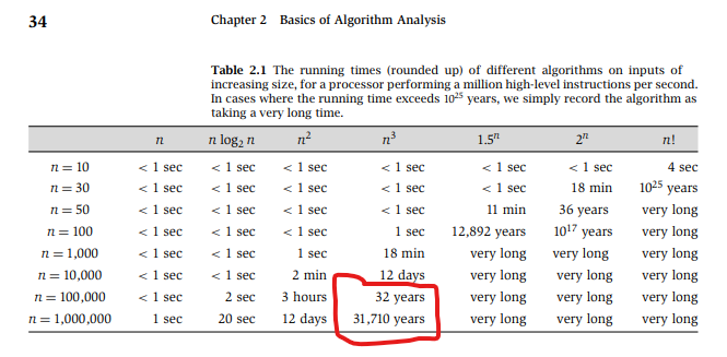
For example, on a computer with a processing speed of 1 MHz (Megahertz) performing 1 million operations per second, there are algorithms with cubic running time n³ that would take 32 years to complete on an input size of 100,000 and over 31,000 years on an input size of 1,000,000, as shown in the figure below.
As we did earlier, let us explore some simple algorithms and their running times.
- Constant time or 1
Example: Accessing an item in an Array given an index.
ACCESSARRAYITEM(arr, index)
1. return arr[index]  # one statement = 1 operation
This algorithm indexes into an array to access the element with the specified index. There is no need to traverse the array. The instruction written above allows the computer to access the memory address of the item in the array instantly, independent of the size of the array.
2. Linear time or n
Example: Finding the maximum item in an array.
FINDMAXITEM(arr)
1. max <- arr[0]
# Assignment statement = 1 operation

2. for i <- 1, to n - 1
# Coding this will look like for(int i = 1; i < n; i++)
# Assignment statement = 1 operation,
# Comparison = 1 operation,
# Increment = 1 operation.
# Total => 3 operations
# Executed (n-1) times => 3*(n-1) => 3n - 3

3.   if arr[i] > max
 # Comparison statement = 1 operation

4.     max = arr[i]
 # Assignment statement = 1 operation

5. return max
# Return statement = 1 operation


# Total running time = 1 + 3n -3 + 1 + 1 + 1 => 3n + 1
The algorithm above finds the maximum element in an array of integers. It takes in the array as an argument, assigns the first element in the array to a variable max, loops through the remaining elements, and compares the element with the value of max. If the element is greater than the value of max, we assign the element to the variable max, making it the new maximum value. At the end of the loop, we return max, the maximum element in the array.
Here is the full algorithm below
FINDMAXITEM(arr)
1. max <- arr[0]
2. for i <- 1, to n - 1
3.   if arr[i] > max
4.     max = arr[i]
5. return max
and implemented in Java
Public int FindMaxItem(int [] arr)
int max = arr[0]
for (int i =1; i < n; i++){
 if (arr[i] > max) max = arr[i]
}
return max
The algorithm has a linear time complexity because the number of operations is directly proportional to the size of the input array n. If there are n elements in the array, the loop iterates n times to find the maximum element.
If the array’s size n is 5, it will take approximately 15 (3n → 3 * 5) operations to find the maximum element. If the array’s size increases to 10, the time complexity increases proportionately to 30 operations. The (1) is a constant because no matter how much n increases, it remains the same. This is why, in complexity analysis, constants are negligible.
3. Quadratic time or n²
Example: Bubble Sort Algorithm to sort an Array.
SORTARRAY(arr)
1. n <- arr.length
# Assignment statement = 1 operation.
# We are assigning the length of the array to a variable n

# OUTER LOOP
2. for i <- 0 to n - 1
    # Assignment = 1 operation. Assigning 0 to the variable i.
    # comparison = 1 operation. Comparing i to n
    # increment = 1 operation. Incrementing i
    # Total = 3 operations
    # Executed (n - 1) times => 3*(n-1) => 3n - 3

# INNER LOOP
3.    for j <- 0 to n - i - 2
      # Assignment = 1, comparison = 1, increment = 1. Total = 3 operations
      # executed (n - 2) times for each n in the outer loop
      # (3 * (n-2)) * n => (3n - 6) * n => 3n² - 6n

4.        if arr[j + 1] < arr[j]
          # Comparison = 1 operation

5.             SWAP(arr[j + 1], arr[j])
               # Typically done in 2 or 3 Assignment statement
               # Hypothetically 3 operations
               # See the python implementation below

6. return arr
   # Return statement = 1 operation

# Total running time = 3n² - 6n + 3n - 3 + 1 + 1 + 1 + 3 = > 3n² - 3n + 3
As the name implies, the bubble sort algorithm is a sorting algorithm. It is perhaps the most common example of an algorithm with a quadratic running time. Here, we are iterating through an array and comparing each item to the other items in the array, which is achieved using a nested loop.
As the size of n increases, the number of operations performed in this algorithm increases quadratically. On an input array of size n = 5, this algorithm would sort the array in about 25 operations (5²).
Here is the full algorithm.
SORTARRAY(arr)
1. n <- arr.length
2. for i <- 0 to n - 1
3.    for j <- 0 to n - i - 2
4.        if arr[j + 1] < arr[j]
5.             SWAP(arr[j + 1], arr[j])
6. return arr
Implemented in python
def bubble_sort(arr):
    n = len(arr)
    for i in range(n):
        for j in range(0, n-i-1):
            if arr[j] > arr[j+1]:
                arr[j], arr[j+1] = arr[j+1], arr[j] #SWAP
    return arr
4. Logarithmic time or log(n)
Example: Binary Search Algorithm to search for a target item in an Array
BINARYSEARCH(arr,target)
1. start<- 0
# Assignment = 1 operation

2. end <- arr.length - 1
# Assignment = 1 operation

3. while start<= end
# Comparison = 1 operation

4.    mid <- (start + end) / 2
      # Addition, Division and Assignment = 3 operations

5.    if arr[mid] == target
      # Comparison = 1 operation
6.        return mid
          # Return = 1 operation, if and only if the target is found.

7.    if arr[mid] < target
      # Comparison = 1
8.        start <- mid + 1
          # Addition +  Assignment = 2 operations,
          # if and only if the target is found.

9.    else
10.       end <- mid - 1
          # Subtraction + Assignment = 1 operation,
          # if and only if the target is found.

11. return -1
 # Return = 1

NOTE:
# The while loop from lines 3 through 10 repeats log(n) times
# where n is the length of the array.

# This happens because the algorithm "halves" the input at each iteration
# until the target element is found.

# For the number of operations inside the loop,
# there can only be one outcome because of the IF statements
# Worst case scenario- the target is at the beginning or end of the array
# That means the input will be divided more times

# We will assume the target is on the right side of the middle element
#  and go with the IF statement with the most number of operations
# (The second IF statement)

# The comparison operation in the first IF statement will still be evaluated,
# if arr[mid] == target
# so we add it to the running time.

# Total running time = 1 + 1 + (1 + 3 + 1 + 2)* log(n) + 1 = 7log(n) + 3
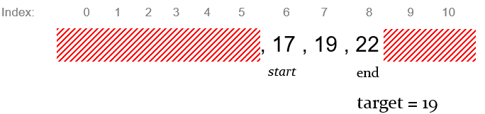
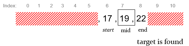
A binary search algorithm takes a sorted array and a search item. We initialize two references/indexes to keep track of the start and the end array. Looping through the array, we find the element in the middle of the array, and if it matches our search, that element is returned.
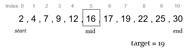
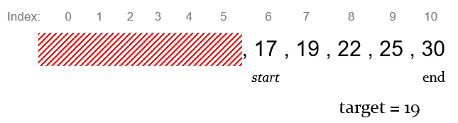
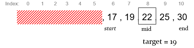
If the target item is larger than the middle element, that means it is on the right side of the middle element. We adjust the start index to the right section of the array, which becomes the new start index for the next iteration of the loop. If the target item is less than the middle element, it exists on the left portion of the array, so we adjust the end index to track the left portion of the array, making it the new end index.
This continues until we find or target element
Here is the full algorithm
BINARYSEARCH(arr,target)
1. start<- 0
2. end <- arr.length - 1
3. while start<= end
4.    mid <- (start + end) / 2
5.    if arr[mid] == target
6.        return mid
7.    if arr[mid] < target
8.        start <- mid + 1
9.    else
10.       end <- mid - 1
11. return -1
Review the Binary Search Algorithm implemented in Python.
def binary_search(arr, target):
    start= 0
    end = len(arr) - 1
    while start <= end:
        mid = (start + end) // 2
        if arr[mid] == target:
            return mid
        elif arr[mid] < target:
            end= mid + 1
        else:
            start = mid - 1
    return -1
Let’s look at the running time 7log(n) + 3. We can say that the time this algorithm takes to find the search item is log(n), ignoring the constant. So if the array size n is 8, then the number of operations log(8) is 3.
Adopting a binary search algorithm to search for an item would make sense given a sorted large dataset. Compared to linear search, binary search is a faster and more efficient algorithm for searching. An input with a size of 32 will take a linear search algorithm 32 operations to search and just 5 for a binary search algorithm.
Conclusion
In summary, we’ve learned about algorithms, their importance, and how to analyze their efficiency through complexity analysis. These tools help us understand how algorithms perform and scale, allowing us to make informed decisions and optimize solutions effectively. In the next episode of this series, we will explore the Big O notation.


