Machine Learning

Tuning Pytorch hyperparameters with Optuna

The post is the fifth in a series of guides to building deep learning models with Pytorch. Below, there is the full series:

1. Pytorch Tutorial for Beginners
2. Manipulating Pytorch Datasets
3. Understand Tensor Dimensions in DL models
4. CNN & Feature visualizations
5. Hyperparameter tuning with Optuna (this post)
6. K Fold Cross-Validation
7. Convolutional Autoencoder
8. Denoising Autoencoder
9. Variational Autoencoder

The goal of the series is to make Pytorch more intuitive and accessible as possible through examples of implementations. There are many tutorials on the Internet to use Pytorch to build many types of challenging models, but it can also be confusing at the same time because there are always slight differences when you pass from one tutorial to another. In this series, I want to start from the simplest topics to the more advanced ones.

Optuna

Optuna is a hyperparameter optimization framework to automate hyperparameter search, which can be applied in Machine Learning and Deep Learning models. Thanks to the fact that it uses sampling and pruning algorithms to optimize the hyperparameters, it’s very fast and efficient. Moreover, it allows for building dynamically the hyperparameter search space in an intuitive way. In this post, I will combine Pytorch and Optuna to find the best-performing CNN model on the MNIST dataset. I will show step by step the functions and the hyperparameters to tune, both needed to apply Optuna.

MNIST classifier with Optuna

We first need to install the library Optuna to make it work:

After, let’s import the libraries and the dataset:

The next step is to define the Convolutional neural network together to the hyperparameters to tune.

In Optuna, the goal is to minimize/maximize the objective function, which takes as input a set of hyperparameters and returns a validation score. For each hyperparameter, we consider a different range of values.

The process of optimization is referred to as a study, while each evaluation of the objective function is called a trial. The “Suggest API” is invoked inside the model architecture to generate dynamically the hyperparameters for each trial.

There are many functions to define the range of the hyperparameters:

• suggest_int suggest integer values for the input units of the second fully connected layer
• suggest_float suggest float values for the dropout rate, introduced as a hyperparameter after the second convolutional layer (0–0.5 with stepsize 0.1) and after the first linear layer (0–0.3 with stepsize 0.1).
• suggest_categorical suggest categorical values for the optimizer, which will be shown later

If you want to check other functionalities, you should look at the documentation here.

I also defined a function to try different values of the batch_size in the training set. It takes as input the training dataset and the batch size, which will be defined later in the objective function, and returns the training and validation loader objects.

Optimization

The most important step is to define the objective function, which uses a sampling procedure to choose the values of the hyperparameters in each trial and returns the validation accuracy obtained in that trial.

After, we can finally create an study object to maximize the objective function. We run the study with study.optimize(objective,n_trials = 20) , where we fix the number of trials equal to 20. You can change it depending on the complexity of the problem.

To have an easier visualization of the hyperparameters chosen in the last 5 trials, we can build a DataFrame object:

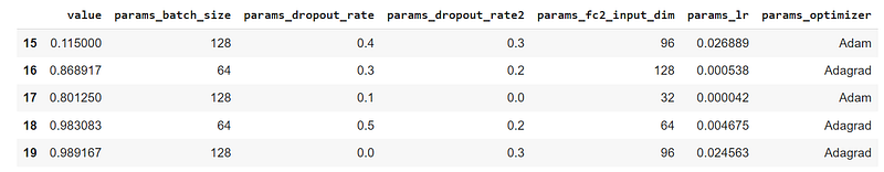
It’s clear that the best-performing model obtained a validation accuracy of 98.9% in the 20th trial. Moreover, you can see the hyperparameter values chosen in that trial.

Visualizations with Optuna

There are many interesting visualizations that help to look at different aspects of the optimization. We can see how the objective value increase as the number of trials increases.

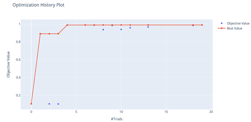
On the x-axis, we have the trials, while on the y-axis there is the objective value, which corresponds to the validation accuracy. With only 20 trials, we can see that we reach good scores above 90%.

We can also show the relationship between different hyperparameters. In this case, we focus only on the batch size and the learning rate:

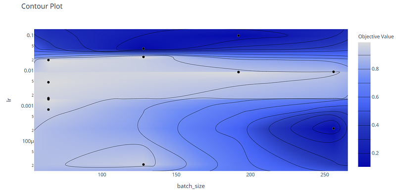
The Contour Plot is a 3D plot, where the third dimension is constituted by the objective value. From the cluster on the center, which is colored in light blue and indicates that there are very high validation accuracies, we can observe that these results are obtained with medium learning rates, between 0.001 and 0.01, and low/medium batch sizes.

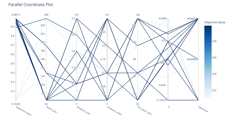
With the Parallel Coordinate plot, we can observe all the optimization history, that has been considered:

Another useful representation is constituted by the hyperparameter importance. So, we are interested to understand which hyperparameters have the highest effect on the performance of the model.

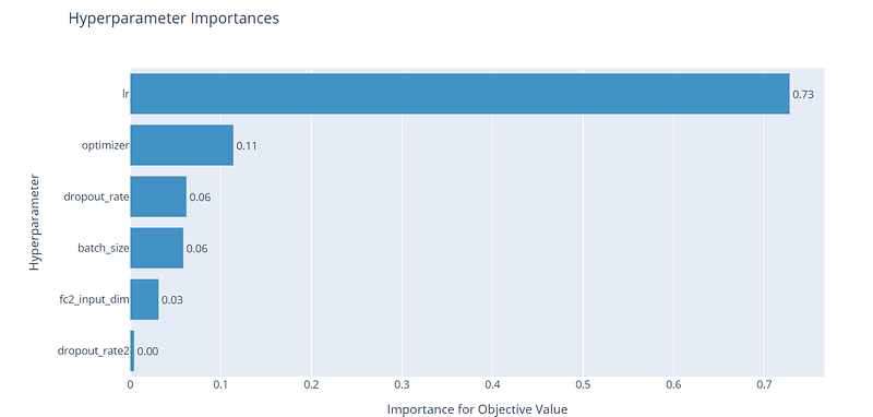
From the plot, we can see that the learning rate has the most huge effect on the objective value, while the rest of the hyperparameters have a very small effect with respect to the learning rate. The dropout rates have a small impact on the performance, but they still are needed to reduce the risk of overfitting.

Final thoughts:

I hope that this post helped you to have an overview of Optuna. I found it very intuitive and fast to use with respect to other methods, like Ray Tune. The GitHub code is here. Thanks for reading. Have a nice day!

Did you like my article? Become a member and get unlimited access to new data science posts every day! It’s an indirect way of supporting me without any extra cost to you. If you are already a member, subscribe to get emails whenever I publish new data science and python guides!