Visualizing the Feature Maps and Filters by Convolutional Neural Networks

A simple guide for interpreting what Convolutional Neural Network is learning using Pytorch

The post is the fourth in a series of guides to building deep learning models with Pytorch. Below, there is the full series:

1. Pytorch Tutorial for Beginners
2. Manipulating Pytorch Datasets
3. Understand Tensor Dimensions in DL models
4. CNN & Feature visualizations (this post)
5. Hyperparameter tuning with Optuna
6. K Fold Cross Validation
7. Convolutional Autoencoder
8. Denoising Autoencoder
9. Variational Autoencoder

The goal of the series is to make Pytorch more intuitive and accessible as possible through examples of implementations. There are many tutorials on the Internet to use Pytorch to build many types of challenging models, but it can also be confusing at the same time because there are always slight differences when you pass from one tutorial to another. In this series, I want to start from the simplest topics to the more advanced ones.

Introduction

The convolutional neural network is a particular type of Artificial Neural Network, widely applied for image recognition. The success of this architecture began in 2015 when the ImageNet image classification challenge was won thanks to this approach.

As you probably know, these methods are very powerful and good in making predictions, but at the same time, they are hard to interpret. For this reason, they are also called black-box models.

There are surely available model-agnostic methods, like LIME and partial dependence plots, that can be applied to any model. But in this case, it makes more sense to apply interpretable methods developed appositely for neural networks. Different from ML models, convolutional neural networks learn abstract features from raw image pixels [1].

In this post, I will focus on how convolutional neural networks learn features. This is possible through visualization of the features learned step by step. Before showing the implementations with Pythorch, I will explain how CNN works and then I will visualize the Feature Maps and the Receptive fields learned by the CNN trained for a classification task.

Table of Content:

1. What is CNN

2. Define and train CNN on MNIST

3. Evaluate model on test set

4. Visualize Filters

5. Visualize Feature Maps

1. What is CNN?

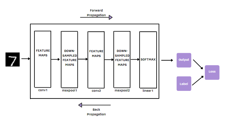
CNNs are made up of building blocks: convolutional layers, pooling layers, and fully connected layers. The main function of the convolutional layer is to extract features or so-called feature maps. How is it able to do it? It uses multiple filters from the dataset [2].

After, the dimensionality of the feature maps from the convolution operation is reduced by the pooling layer. The most used pooling operation is Maxpooling, which selects the most significant pixel value in each filter patch of the feature map. So, these two types of layers are useful to perform feature extraction.

Differently from convolutional and pooling layers, the fully connected layer maps the extracted features into the final output, for example, the classification of MNIST’s image as one of the 10 digits.

In digital images, a two-dimensional grid stores the pixel values. It can be seen as an array of numbers. The kernel, which is a small grid, typically with size 3x3, is applied at each position of the image. As you go into deeper layers, the features are becoming progressively more and more complex.

The model’s performance is obtained with a loss function, which is the difference between outputs and target labels, through forward propagation on the training set, and parameters, such as weights and bias, are updated through backpropagation with the gradient descent algorithm.

2. Define and Train CNN on MNIST dataset

Let’s first import the libraries and the dataset. torch is the module that provides data structures for tensors with one or more dimensions.

The most important libraries are:

• torchvision consists of popular datasets, famous model architectures, and common image transformations. In our case, it provides us with the MNIST dataset.
• torch.nn contains classes and functions that will help you to build the Convolutional Neural Network.
• torch.optim provides all the optimizers such as Adam.
• torch.nn.functional is used to import functions, such as dropout, convolution, pooling, non-linear activation functions, and loss functions.

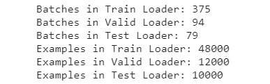
We download the training and the test datasets and we transform the image datasets into Tensor. We don’t need to normalize the images because the datasets contain already grayscale images. After we divide the training dataset into training and validation sets.The random_split provides a random partition for these two sets. The DataLoader is used to create data loaders for the training, validation, and test sets, which are split into mini-batches. The batchsize is the number of samples used in one iteration during the training of the model.

We define CNN architecture.

We can print the CNN easily to have a fast overview:

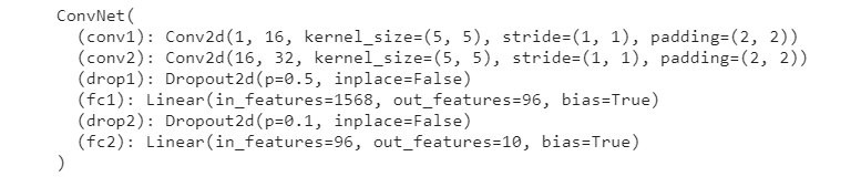
You can see that there are two convolutional layers and two fully connected layers. Each convolutional layer is followed by the ReLU activation function and max-pooling layer. The view function reshapes the data into a one-dimensional array, that will be passed to the linear layer. The second fully connected layer, also called the output layer, will classify the image as one of the 10 digits.

We define the building blocks, that will be used to train the CNN:

• torch.device to train the model with a hardware accelerator like the GPU
• CNN network, that will be moved to the device
• Cross Entropy Loss and Adam optimizer

Now, we can train the network on the training set and evaluate it on the validation set:

The training code can be broken into two parts.

Forward Propagation:

1. We pass the input images to the network with model(images)
2. The loss is computed by calling criterion(outputs,labels) where outputs constitute the predicted class and labels constitute the target class.

Back Propagation:

3. The gradient is cleared to be sure we don’t accumulate other values with optimizer.zero_grad()

4. loss.backward() is used to perform Back Propagation and calculates the gradient based on the loss

5. optimizer.step() is always after the computation of the gradient. It iterates over all the parameters and updates their values.

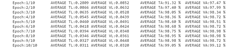
The loss function and accuracy are calculated for both training and validation sets.

3. Evaluate model on test set

Once the model is trained, we can evaluate the performance on the test set:

Let’s break the test code into little pieces:

• torch.no_grad() is used to disable the Gradient Tracking, we don’t need the compute the gradients anymore since the model is already trained
• pass the input images to the network
• calculate the test loss by adding loss.item()*images.size(0)
• calculate the test accuracy by adding (predicted==labels).sum().item()

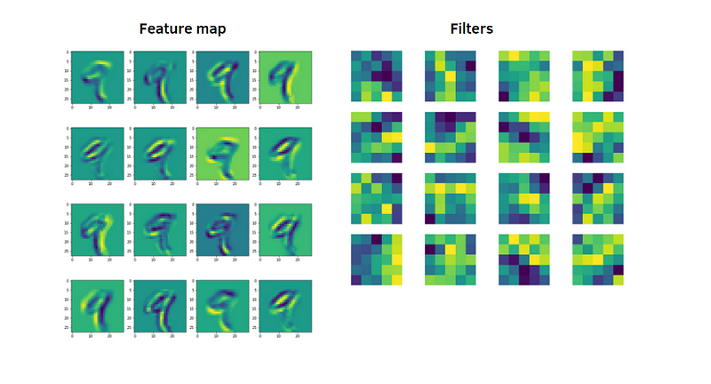
4. Visualize Filters

We can visualize the learned filters, used by CNN to convolve the feature maps, that contain the features extracted, from the previous layer. It’s possible to obtain these filters by iterating through all the layers of the models, list(model.children()). If the layer is convolutional, we can store the weight in the list model_weights, which will contain the filters used in the two convolutional layers.

Below I show the shape of the filters found.

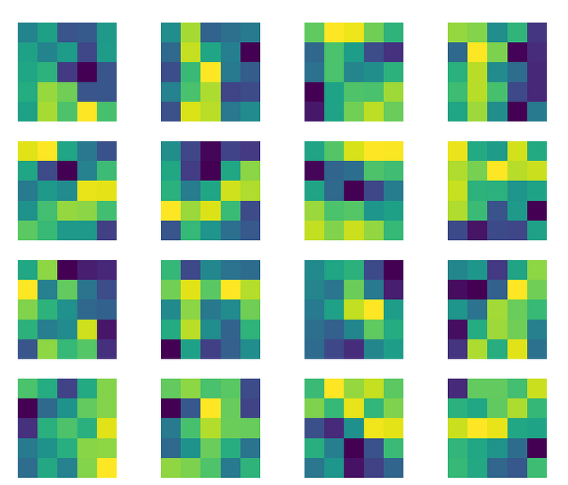
Now, we can finally visualize the learned filters of the first convolution layer:

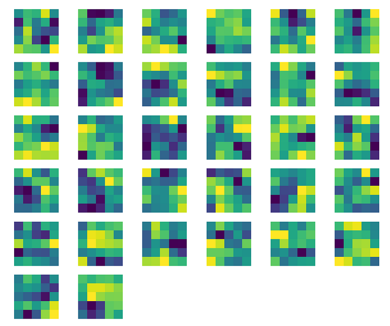
Now, it’s the turn to visualize the filters of the second convolutional layer.

5. Visualize Feature Maps

The Feature Map, also called Activation Map, is obtained with the convolution operation, and applied to the input data using the filter/kernel. Below, we define a function to extract the features obtained after applying the activation function.

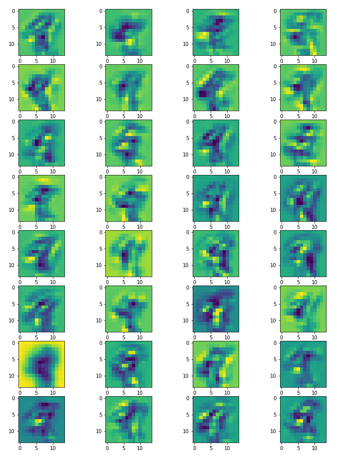
From the training dataset, we take an image that represents the digit 9. So, we’ll visualize the feature maps obtained for that image in the first convolutional layer.

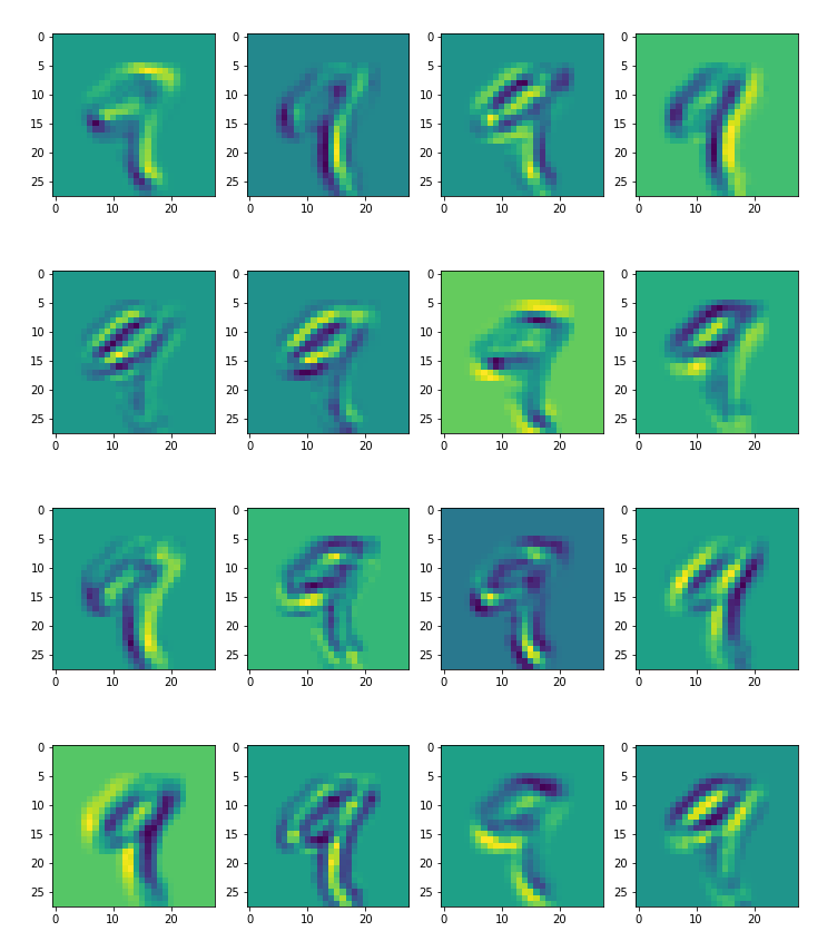
Now, we visualize the feature maps obtained for the same image in the second convolutional layer.

Final thought:

Congratulations! You have learned to visualize the learned features by CNN with Pytorch. The network learns new and increasingly complex features in its convolutional layers. From the first convolutional layer to the second convolutional layer, you can see the differences in these features. The more you go further in the convolutional layers, the more the features will be abstract. The GitHub code is here. Thanks for reading. Have a nice day.

References:

[1] https://christophm.github.io/interpretable-ml-book/cnn-features.html#feature-visualization

[2] https://insightsimaging.springeropen.com/articles/10.1007/s13244-018-0639-9

Did you like my article? Become a member and get unlimited access to new data science posts every day! It’s an indirect way of supporting me without any extra cost to you. If you are already a member, subscribe to get emails whenever I publish new data science and python guides!