The Same, or Not the Same — That is the Problem of Entity Resolution

Four methods for finding identical or similar entities in biomedical and customer data

Humans are highly skilled at discerning whether two things are identical or not. For instance, we know that HIV and Human Immunodeficiency Virus refer to the same virus. But we also know that Jimmy Kimmel and Jimmy Fallon are not the same person, even though they have similar names and share the same profession. The process of identifying and linking the same entities is called entity resolution.

Entity resolution can be seen as a special case of classification in machine learning. It is a fundamental process, especially for knowledge graph construction, fraud detection, and customer relationship management. On the one hand, different people can name the same thing differently, even within the same organization. On the other hand, we often group similar entities together so that we can understand them better as a whole. For example, we can group addresses together into a district so that we can calculate its average house price or crime rate.

Entity recognition can be quite challenging for computers, as it requires the system to understand the context of unstructured data and to identify the patterns that are associated with different types of entities. In the book Building Knowledge Graphs, Barrasa et al. used strong identifiers, weak identifiers, Weakly Connected Components (WCC) algorithm, and natural language processing (NLP) to connect identical or similar entities in graphs. In my previous article From Raw Text to Wikidata Taxonomy and Knowledge Graph, I used GCP’s Natural Language AI to extract named entities from raw texts (NER), linked them to the Wikidata ontology, and unified the coreferences.

These methods are effective for data with identifiers (e.g., social security numbers, driver’s license numbers) or news articles. However, they are not sufficient for many scientific or enterprise applications. Different fields often have different domain-specific entity resolutions. For example, in biology, we are dealing with DNA or protein sequences, disease names, Linnaean taxonomy, and other technical terms. In banking or other customer applications, we need to cluster people based on their addresses. In this short article, I would like to show you my entity resolutions in these applications. The code for this project is hosted on my GitHub here.

1. Biomedicine

There are many different types of data in biomedicine, including DNA and protein sequences, disease and organism names. Bioinformaticians have developed specific methods to compare and identify these entities.

1.1 DNA sequences

DNA sequencing reads the nucleotide (A, T, C, and G) sequence of the DNA molecules. The technology has experienced a rapid transformation in recent years. Sequencing throughput has increased exponentially, while its cost has come down dramatically. With this powerful technology, biologists worldwide are sequencing everything they can get their hands on, microorganisms, macroorganisms, and metagenomes. As a result, a deluge of DNA sequences has stormed the public databases. Although many of those sequences are completely unique and novel, some of them do share similarities with those in the databases. In bioinformatics, we align DNA sequences against each other and find the so-called hits — sequences that are identical with or similar to the query sequences. One of the best-known and most widely used methods is BLAST. This perennial tool has served the bioinformatic community since 1990 (1). It compares your input sequence against a sequence database and returns the hits.

You can run BLAST locally, on the NCBI website, in a cluster, or on the cloud. In Figure 1, you can see that I was BLASTing a random GH43 gene against the nt_euk database in NCBI. It turned out to be identical to the gene LCP9604111_1709 from the genome of Penicillium roqueforti strain LCP96 04111.

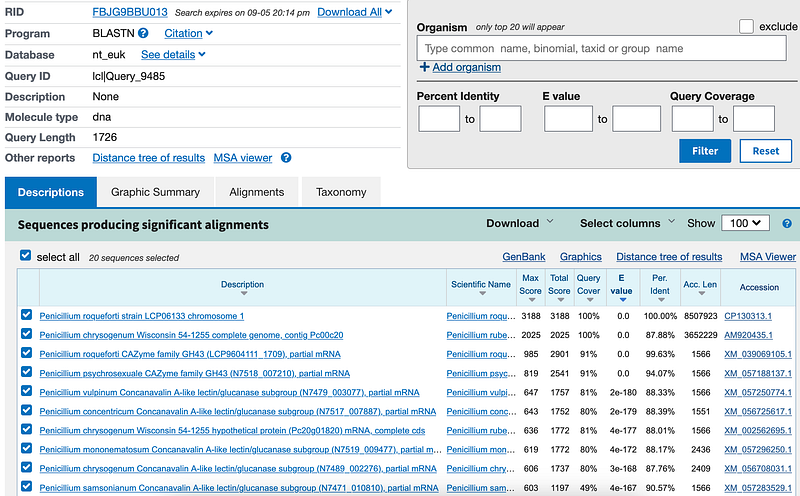
As you can see, the first hit was an identical match. The subsequent hits were not perfect matches and were thus called similar sequences. The user need to decide to what extent a sequence can still be considered similar. For example, homology is typically defined as a sequence identity of at least 30% (1).

We can also group sequences without matching them against any external database. This is called clustering in the bioinformatic parlance. For this purpose, we can use CD-HIT, VSEARCH, and some others. These tools will output clusters of sequences that resemble each other.

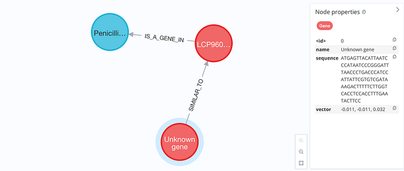
Once we define and obtain similar sequences, we can construct a knowledge graph based on the results (Figure 2). This knowledge graph represents the newly sequenced DNA samples and their database hits. After entity resolution, we can learn the approximate taxonomic composition of our samples. Furthermore, sometimes sequence similarity implies functional similarity. It is therefore possible to get a coarse overview of the functional diversity in the samples as well.

1.2 Protein sequences

If DNA is the recipe, then protein is the dish. Biochemically, the DNA sequence determines the amino acid sequence in a protein, which is also called its primary structure. To some extent, we can compare proteins in the same way that we compare DNA. However, the molecular function of a protein is determined more by its shape than its amino acid sequence. Some similar protein sequences can have different shapes and consequently different functions. A good example is the beta-globin. Just one particular mutation among its 600 amino acids can alter the protein surface structure. And it can ultimately lead to Sickle cell disease (SCD).

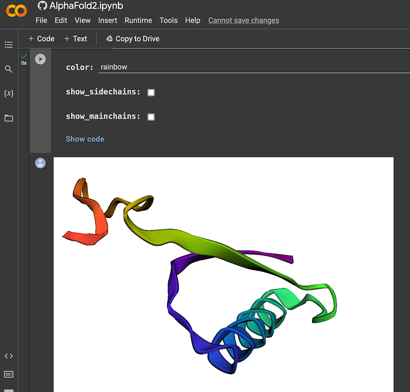
Determining the structures of proteins was a time-consuming and laborious process in the past. It was a major computational challenge, too. This has changed since the sensational debut of AlphaFold (Figure 3). AlphaFold is able to predict the 3D structure of a protein based on its amino acid sequence with much better accuracy than its predecessors. With a tool like VAST Search (Figure 4) from NCBI, it is possible to find similar proteins based on their structures by purely geometric criteria.

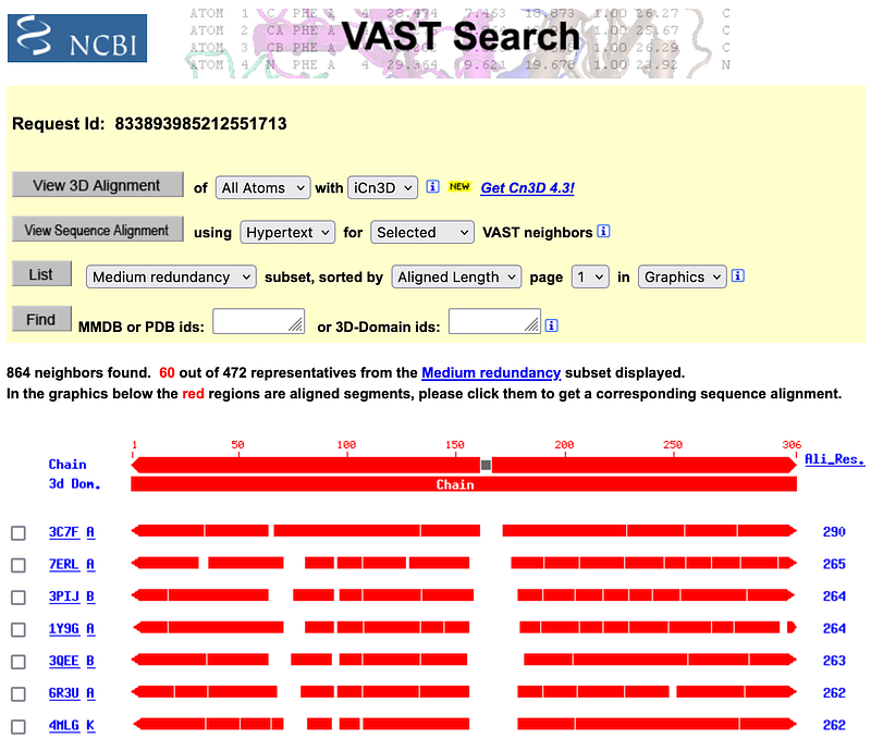
3D structural comparison has some advantages over sequence-based methods. Similar sequences can sometimes form very dissimilar structures. A 3D structural search can thus identify distant homologs that cannot be recognized by sequence comparison alone.

1.3 Medical concepts

Bioinformaticians are also increasingly working with natural language data, which includes research articles, health records, and other unstructured raw texts. The texts first need to go through a series of preprocessing steps, including coreference resolution, relationship extraction, and entity resolution. In my previous article From Raw Text to Wikidata Taxonomy and Knowledge Graph, I demonstrated a pipeline based on GCP, GPT, and Wikidata that can fulfill these functions. However, biomedical literature is often full of technical terms and requires specific vocabulary and ontology services, such as the NCBI Taxonomy, SNOMED, and more generally, the Unified Medical Language System (UMLS).

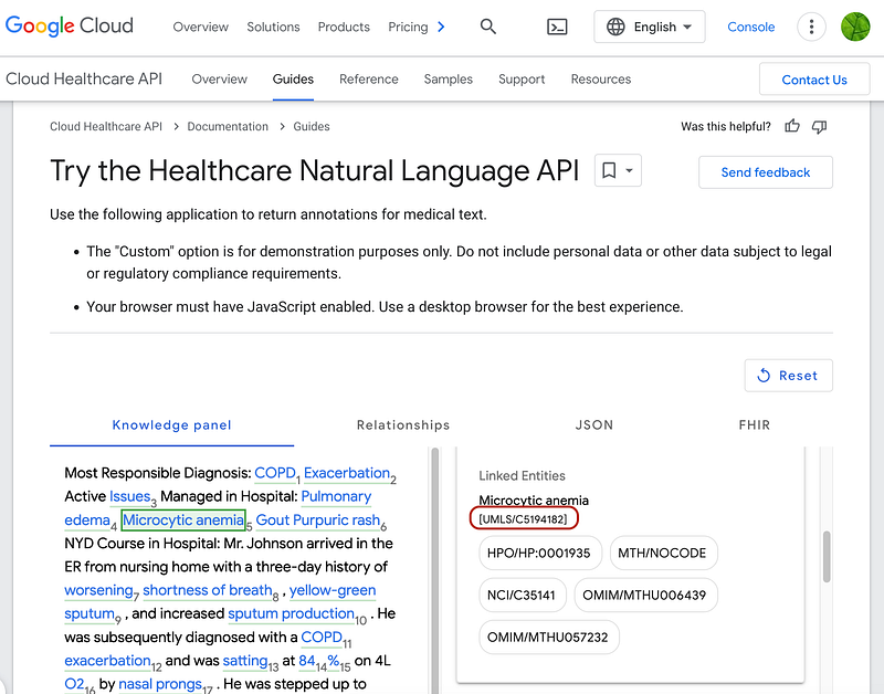
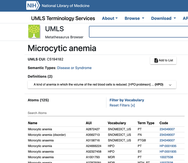
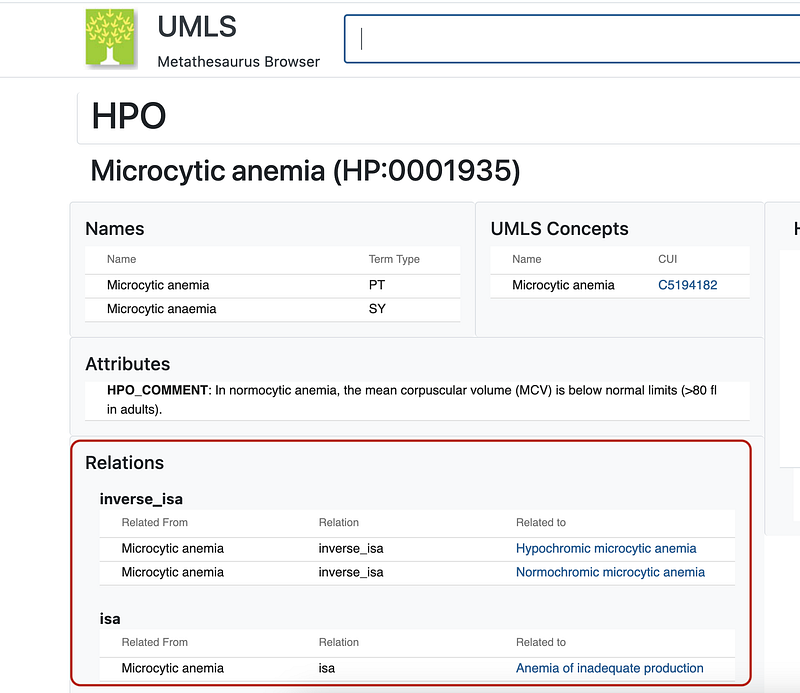
I have previously written tutorials about the first two (Serve NCBI Taxonomy in AWS, Serverlessly for NCBI Taxonomy, and Clinical Trials as Graphs and Vectors for SNOMED). UMLS maps biomedical terms across different vocabularies. We can start by using Google’s Cloud Healthcare API to extract entities from biomedical raw texts. More importantly, the Healthcare API annotates the entities with their UMLS IDs (Left panel in Figure 5). We can then query NIH’s UMLS Terminology Services with these IDs and find their links in other vocabularies (Middle panel in Figure 5). Human Phenotype Ontology (HPO) is one of such vocabularies. Figure 5 demonstrates that the Healthcare API extracts many medical terms from the example text. Among them, microcytic anemia has been annotated with the UMLS ID C5194182. This ID helped me find the entry “Microcytic anemia” on UMLS’ page (Middle panel in Figure 5). The HPO service then revealed its taxonomic relationships (Right panel in Figure 5). For example, “Microcytic anemia” has an “is a” relationship with “Anemia of inadequate production”.

2. Addresses

Fraud is a big problem and costs a lot. According to TigerGraph, not only funds and goods are directly stolen from customers and vendors, but various industries also need to spend time and money on fighting it. Finally, these measures and countermeasures have a negative impact on the customer experience and thus reduce the so-called customer lifetime value.

Computer scientists have developed several fraud detection methods for transactional data. Some rely on big data and others are based on graphs. According to this video from TigerGraph, one of the detection methods is called deep link analytics. It identifies transactions that form closed loops in the graph. In TigerGraph’s example, the doctor was colluding with the administrator. By analyzing their addresses, the investigators realized that the two were neighbors and thus connected them in the graph to form a closed loop. This closed loop was the first hint about their collusion. This address analysis can be considered as a form of entity resolution. It starts with a set of addresses, sets a distance threshold, and classifies the neighbors. TigerGraph does not mention how it implemented this analysis in the post. But I can use Google’s Geocoding API to do the same. Let’s say we have the following set of addresses (Table 1).

As you can see in Table 1, based on the address strings alone, it is quite challenging for us and for the computer to identify the neighbors (< 50m from each other). Let’s calculate the distance with the following Python script.

import googlemaps
import mpu

gmaps = googlemaps.Client(key=PARAM["GOOGLE_API_KEY"])

addresses = pd.read_csv("address.tsv", sep="\t")

# get the lat,lon from Google's geocode API
for index, row in addresses.iterrows():
    geocode_result = gmaps.geocode(row["address"]) 
    lat = geocode_result[0]["geometry"]["location"]["lat"]
    lng = geocode_result[0]["geometry"]["location"]["lng"]

    addresses.loc[index, "lat"] = lat
    addresses.loc[index, "lng"] = lng

# pairwise combinations of the addresses
idxs = list(combinations(addresses.index,2))
dfx = pd.DataFrame(np.concatenate((addresses.iloc[idx[0]].values, addresses.iloc[idx[1]].values)) for idx in idxs)
dfx.columns = ['s_name', 's_address', 's_lat', 's_lng', 'd_name', 'd_address', 'd_lat', 'd_lng']

# Calculate the Haversine distance from the mpu library
for index, row in dfx.iterrows():
    dist = mpu.haversine_distance((row["s_lat"], row["s_lng"]), (row["d_lat"], row["d_lng"]))
    dfx.loc[index, "distance"] = dist

## output
#s_name .. d_name .. distance
#A .. B .. 0.025376
#A .. C .. 22.902873
#A .. D .. 0.109389
..

# Get neighbor addresses that are less than 50m from each other
dfx[dfx["distance"] < 0.05]

## output
#s_name .. d_name .. distance
#A .. B .. 0.025376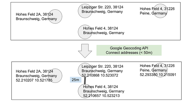

The code is straightforward. It gets the addresses and sends them to Google’s Geocoding API. The API returns the coordinates. Then the program uses the mpu package to calculate the pairwise Haversine distances. Addresses within 50 meters of each other are considered neighbors (Figure 6). We can then connect these neighbors in the graph and run the deep link analytics ourselves. However, the script does a pairwise comparison among the addresses. And that will become expensive for large datasets. We can consider clustering the addresses first and only compute the distances for pairs from the same region. But such a method will miss neighbors across the region boundaries.

Conclusion

Relationships are first-class citizens in graphs. But if synonymous nodes are not resolved, they will divert the relationships. Entity resolution can thus improve the graph by removing this kind of ambiguity. After identifying identical or similar nodes, we can redirect the links to the master entities. The resulting graph becomes more consistent. Both the maintainers and the users will find it easier to understand the graph, too.

However, entity resolution is a reoccurring task. As new data comes, it needs to be performed again to ensure the unambiguity. There are attempts to automate the process. For example, the GRAPE (Graph Representation leArning, Predictions and Evaluation) library can do densification or link prediction on a graph. Its similarity search is based on either the external Wikipedia descriptions or the internal node properties. Certainly, we can use such functions to connect identical or similar nodes in some use cases. However, these libraries cannot perform the entity resolutions shown in this article. Different domains may require different automatic workflows. They require the participation of domain experts, linguists, and programmers.

So what kind of entity resolution do you perform for your graphs?