Stable Diffusion Clearly Explained!

How does Stable Diffusion paint an AI artwork? Understanding the tech behind the rise of AI-generated art.

Most of the recent AI art found on the internet is generated using the Stable Diffusion model. Since it is an open-source tool, any person can easily create fantastic art illustrations from just a text prompt.

In this article, I’m going to explain how it works.

Table of Contents

- Diffusion Model — Forward Diffusion Process — Reverse Diffusion Process — Training — Sampling — Diffusion Speed Problem - Stable Diffusion — Departure to Latent Space — Latent Diffusion — Conditioning — Training — Sampling - Architecture Comparison — Pure Diffusion Model — Stable Diffusion (Latent Diffusion Model) - Summary - FurtherReading: Advanced Conditioning - References

Diffusion Model

If you want to understand the full details of the Diffusion Model, you can check out my previous article:

Here I will walk you through the rough idea of the Diffusion Model.

The training of the Diffusion Model can be divided into two parts:

1. Forward Diffusion Process → add noise to the image.
2. Reverse Diffusion Process → remove noise from the image.

Forward Diffusion Process

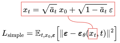
The forward diffusion process adds Gaussian noise to the input image step by step. Nonetheless, it can be done faster using the following closed-form formula to directly get the noisy image at a specific time step t:

Reverse Diffusion Process

Since the reverse diffusion process is not directly computable, we train a neural network εθ to approximate it.

The training objective (loss function) is as follows:

Training

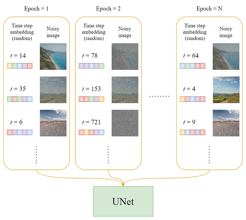
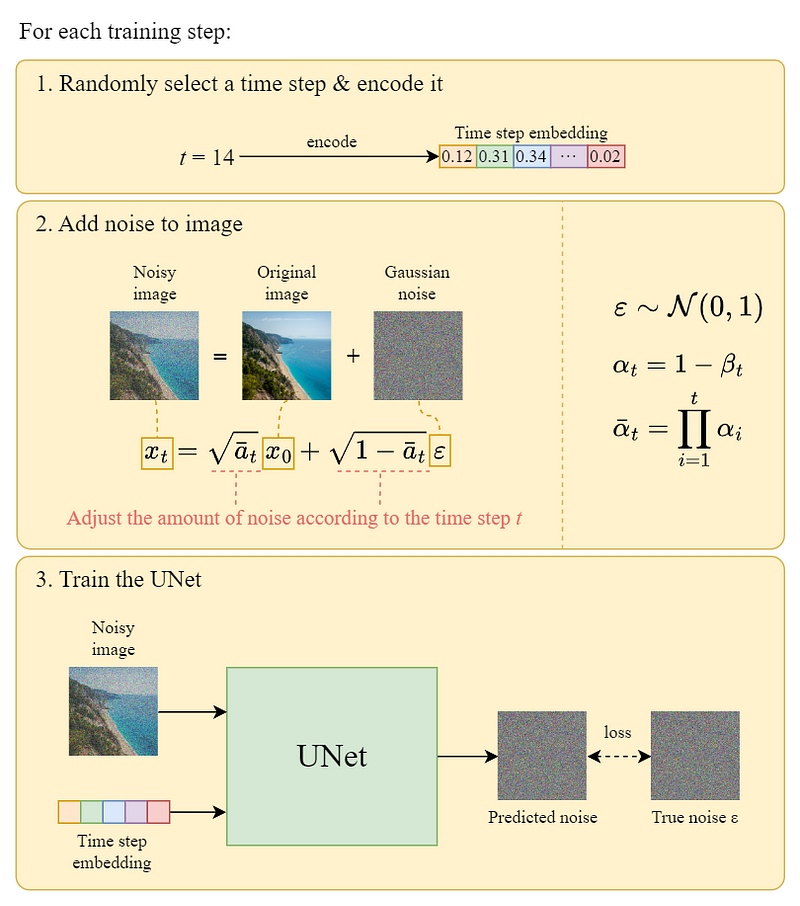
In each epoch:

1. A random time step t will be selected for each training sample (image).
2. Apply the Gaussian noise (corresponding to t) to each image.
3. Convert the time steps to embeddings (vectors).

Sampling

Sampling means painting an image from Gaussian noise. The following diagram shows how we can use the trained U-Net to generate an image:

Diffusion Speed Problem

As you can see, the diffusing (sampling) process iteratively feeds a full-sized image to the U-Net to get the final result. This makes the pure Diffusion model extremely slow when the number of total diffusing steps T and the image size are large.

Hereby, Stable Diffusion is designed to tackle this problem.

Stable Diffusion

The original name of Stable Diffusion is “Latent Diffusion Model” (LDM). As its name points out, the Diffusion process happens in the latent space. This is what makes it faster than a pure Diffusion model.

Departure to Latent Space

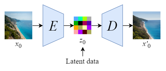
We will first train an autoencoder to learn to compress the image data into lower-dimensional representations.

• By using the trained encoder E, we can encode the full-sized image into lower dimensional latent data (compressed data).
• By using the trained decoder D, we can decode the latent data back into an image.

Latent Diffusion

After encoding the images into latent data, the forward and reverse diffusion processes will be done in the latent space.

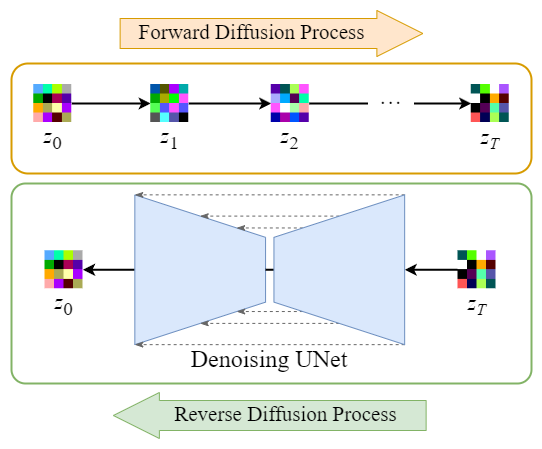
1. Forward Diffusion Process → add noise to the latent data.
2. Reverse Diffusion Process → remove noise from the latent data.

Conditioning

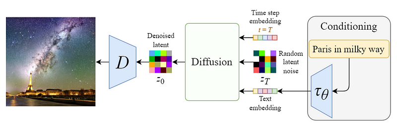
The true power of the Stable Diffusion model is that it can generate images from text prompts. This is done by modifying the inner diffusion model to accept conditioning inputs.

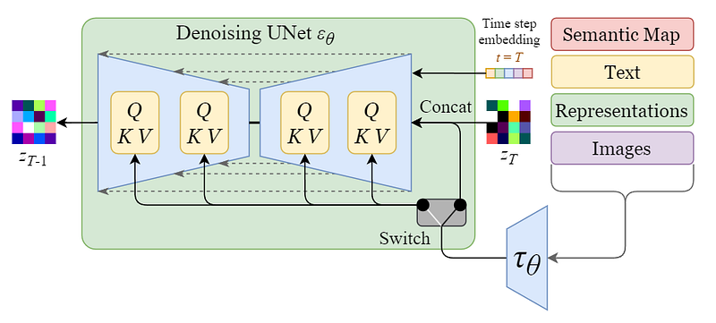
The inner diffusion model is turned into a conditional image generator by augmenting its denoising U-Net with the cross-attention mechanism.

The switch in the above diagram is used to control between different types of conditioning inputs:

• For text inputs, they are first converted into embeddings (vectors) using a language model 𝜏θ (e.g. BERT, CLIP), and then they are mapped into the U-Net via the (multi-head) Attention(Q, K, V) layer.
• For other spatially aligned inputs (e.g. semantic maps, images, inpainting), the conditioning can be done using concatenation.

Training

The training objective (loss function) is pretty similar to the one in the pure diffusion model. The only changes are:

• Input latent data zₜ instead of the image xₜ.
• Added conditioning input 𝜏θ(y) to the U-Net.

Sampling

Since the size of the latent data is much smaller than the original images, the denoising process will be much faster.

Architecture Comparison

Finally, let’s compare the overall architectures of the pure diffusion model and the stable diffusion model (latent diffusion model).

Pure Diffusion Model

Stable Diffusion (Latent Diffusion Model)

Summary

To quickly summarize:

• Stable Diffusion (Latent Diffusion Model) conducts the diffusion process in the latent space, and thus it is much faster than a pure diffusion model.
• The backbone diffusion model is modified to accept conditioning inputs such as text, images, semantic maps, etc.

Further Reading: Advanced Conditioning

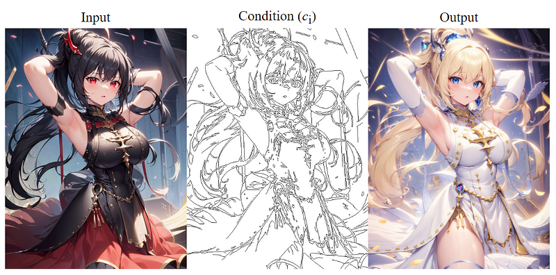
By using ControlNet alongside Stable Diffusion, you can generate the image from other types of conditioning images, e.g. canny edge.

References

[1] R. Rombach, A. Blattmann, D. Lorenz, P. Esser, and B. Ommer, “High-resolution image synthesis with Latent Diffusion Models,” arXiv.org, 13-Apr-2022. [Online]. Available: https://arxiv.org/abs/2112.10752.

[2] J. Alammar, “The Illustrated Stable Diffusion,” The Illustrated Stable Diffusion — Jay Alammar — Visualizing machine learning one concept at a time. [Online]. Available: https://jalammar.github.io/illustrated-stable-diffusion/.

[3] A. Gordić, “Stable diffusion: High-resolution image synthesis with latent diffusion models | ML coding series,” YouTube, 01-Sep-2022. [Online]. Available: https://www.youtube.com/watch?v=f6PtJKdey8E.