Diffusion Model Clearly Explained!

How does AI artwork work? Understanding the tech behind the rise of AI-generated art.

Jason Allen’s AI-generated work, “Théâtre D’opéra Spatial,” won first place in the digital category at the Colorado State Fair. [1]

The rise of the Diffusion Model can be regarded as the main factor for the recent breakthrough in the AI generative artworks field.

In this article, I’m going to explain how it works with illustrative diagrams.

Updates

[15-Jun-2023] Added detailed derivation of the mean μ̃ₜ of q(xₜ₋₁|xₜ, x₀) for the stepwise denoising term in Loss Function.

- Overview - Forward Diffusion Process — Closed-Form Formula - Reverse Diffusion Process — Loss Function — Simplified Loss - The U-Net Model — Dataset — Training — Reverse Diffusion - Summary - Appendix - References

Overview

The training of the Diffusion Model can be divided into two parts:

Forward Diffusion Process → add noise to the image.
Reverse Diffusion Process → remove noise from the image.

Forward Diffusion Process

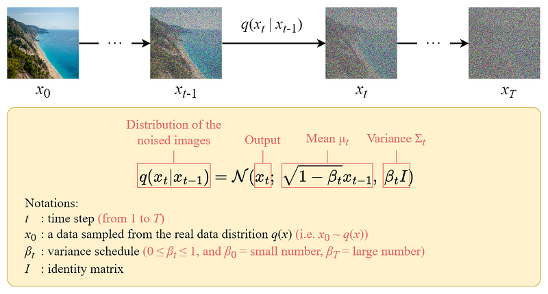
The forward diffusion process gradually adds Gaussian noise to the input image x₀ step by step, and there will be T steps in total. the process will produce a sequence of noisy image samples x₁, …, x_T.

When T → ∞, the final result will become a completely noisy image as if it is sampled from an isotropic Gaussian distribution.

But instead of designing an algorithm to iteratively add noise to the image, we can use a closed-form formula to directly sample a noisy image at a specific time step t.

Closed-Form Formula

The closed-form sampling formula can be derived using the Reparameterization Trick.

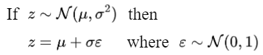
With this trick, we can express the sampled image xₜ as follows:

Express xₜ *using the reparameterization trick*

Then we can expand it recursively to get the closed-form formula:

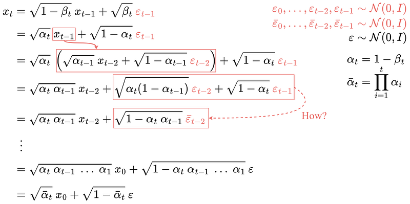
Note: all the ε are i.i.d. (independent and identically distributed) standard normal random variables.

It is important to distinguish them using different symbols and subscripts because they are independent and their values could be different after sampling.

But how do we jump from line 4 to line 5?

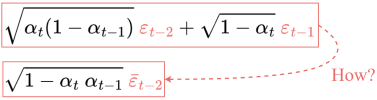
Some people find this step difficult to understand. Here I will show you how it works:

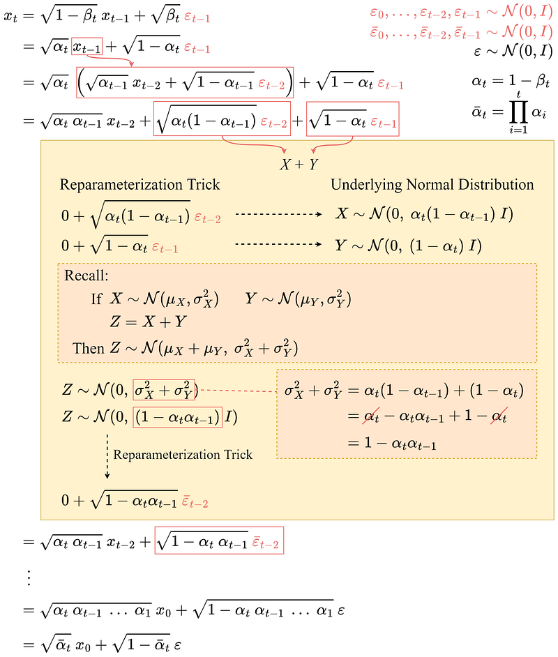
Detailed derivation from line 4 to line 5

Let’s denote these two terms using X and Y. They can be regarded as samples from two different normal distributions. i.e. X ~ N(0, αₜ(1-αₜ₋₁)I) and Y ~ N(0, (1-αₜ)I).

Recall that the sum of two normally distributed (independent) random variables is also normally distributed. i.e. if Z = X + Y, then Z ~ N(0, σ²ₓ+σ²ᵧ).

Therefore we can merge them together and express the merged normal distribution in the reparameterized form. This is how we combine the two terms.

Repeating these steps will give us the following formula which depends only on the input image x₀:

Now we can directly sample xₜ at any time step using this formula, and this makes the forward process much faster.

Reverse Diffusion Process

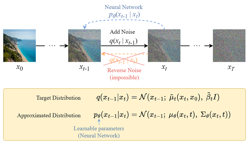
Unlike the forward process, we cannot use q(xₜ₋₁|xₜ) to reverse the noise since it is intractable (uncomputable).

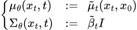
Thus we need to train a neural network pθ(xₜ₋₁|xₜ) to approximate q(xₜ₋₁|xₜ). The approximation pθ(xₜ₋₁|xₜ) follows a normal distribution and its mean and variance are set as follows:

Loss Function

We can define our loss as a Negative Log-Likelihood:

This setup is very similar to the one in VAE. instead of optimizing the intractable loss function itself, we can optimize the Variational Lower Bound.

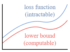
By optimizing a computable lower bound, we can indirectly optimize the intractable loss function.

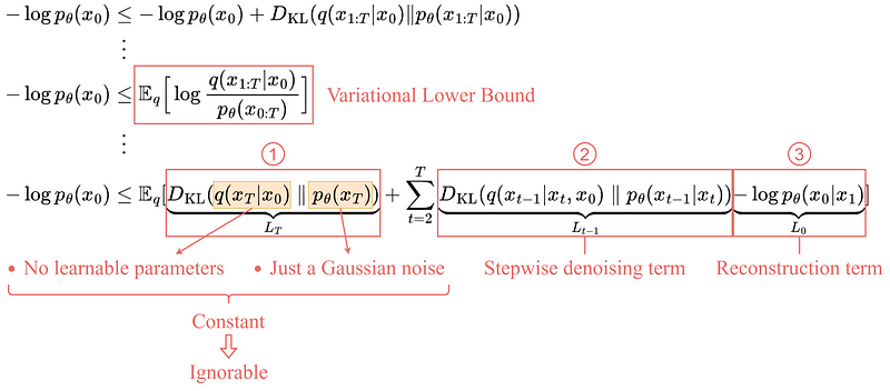
Derivation and expansion of the Variational Lower Bound

By expanding the variational lower bound, we found that it can be represented with the following three terms:

1. L_T: Constant term

Since q has no learnable parameters and p is just a Gaussian noise probability, this term will be a constant during training and thus can be ignored.

2. Lₜ₋₁: Stepwise denoising term

This term compares the target denoising step q and the approximated denoising step pθ.

Note that by conditioning on x₀, the q(xₜ₋₁|xₜ, x₀) becomes tractable.

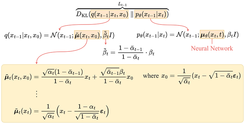
After a series of derivations, the mean μ̃ₜ of q(xₜ₋₁|xₜ, x₀) is shown above.

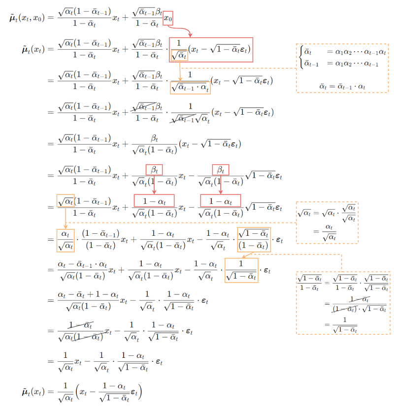
For those who want to see the step-by-step derivation of the mean μ̃ₜ (yellow box), please see the Appendix.

To approximate the target denoising step q, we only need to approximate its mean using a neural network. So we set the approximated mean μθ to be in the same form as the target mean μ̃ₜ (with a learnable neural network εθ):

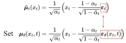
The comparison between the target mean and the approximated mean can be done using a mean squared error (MSE):

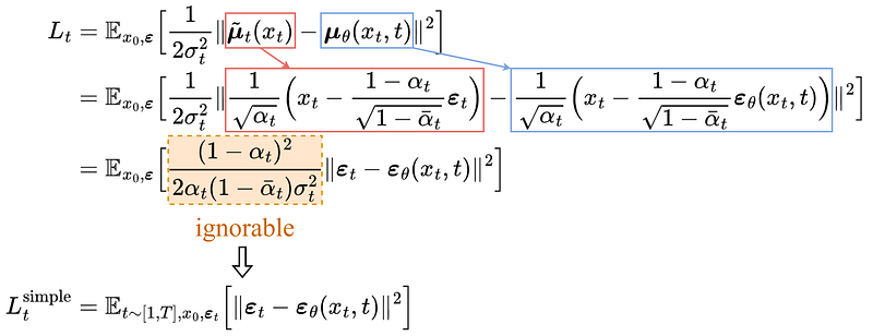
Derivation of the simplified stepwise denoising loss

Experimentally, better results can be achieved by ignoring the weighting term and simply comparing the target and predicted noises with MSE.

So, it turns out that to approximate the desired denoising step q, we just need to approximate the noise εₜ using a neural network εθ.

3. L₀: Reconstruction term

This is the reconstruction loss of the last denoising step and it can be ignored during training for the following reasons:

It can be approximated using the same neural network in Lₜ₋₁.
Ignoring it makes the sample quality better and makes it simpler to implement.

Simplified Loss

So the final simplified training objective is as follows:

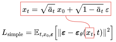
We find that training our models on the true variational bound yields better codelengths than training on the simplified objective, as expected, but the latter yields the best sample quality. [2]

The U-Net Model

Dataset

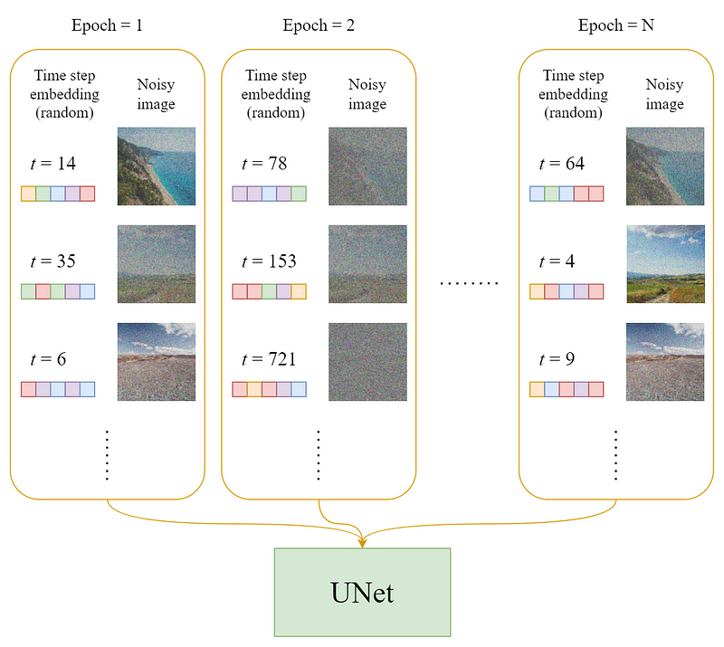
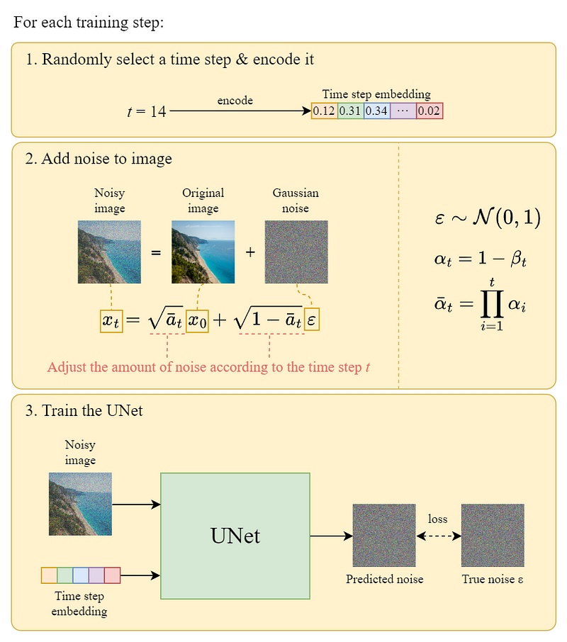
In each epoch:

A random time step t will be selected for each training sample (image).
Apply the Gaussian noise (corresponding to t) to each image.
Convert the time steps to embeddings (vectors).

Training

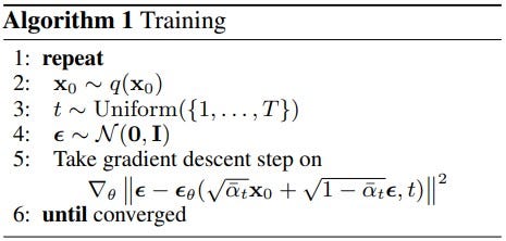
The official training algorithm is as above, and the following diagram is an illustration of how a training step works:

Reverse Diffusion

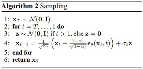
We can generate images from noises using the above algorithm. The following diagram is an illustration of it:

Note that in the last step, we simply output the learned mean μθ(x₁, 1) without adding the noise to it.

Summary

Here are some main takeaways from this article:

The Diffusion model is divided into two parts: forward diffusion and reverse diffusion.
The forward diffusion can be done using the closed-form formula.
The backward diffusion can be done using a trained neural network.
To approximate the desired denoising step q, we just need to approximate the noise εₜ using a neural network εθ.
Training on the simplified loss function yields better sample quality.

Appendix

The following is the detailed derivation of the mean μ̃ₜ of q(xₜ₋₁|xₜ, x₀) in the stepwise denoising term in the Loss Function section.

References

[1] K. Roose, “An a.i.-generated picture won an art prize. artists aren’t happy.,” The New York Times, 02-Sep-2022. [Online]. Available: https://www.nytimes.com/2022/09/02/technology/ai-artificial-intelligence-artists.html.

[2] J. Ho, A. Jain, and P. Abbeel, “Denoising Diffusion Probabilistic models,” arXiv.org, 16-Dec-2020. [Online]. Available: https://arxiv.org/abs/2006.11239.

[3] N. A. Sergios Karagiannakos, “How diffusion models work: The math from scratch,” AI Summer, 29-Sep-2022. [Online]. Available: https://theaisummer.com/diffusion-models.

[4] L. Weng, “What are diffusion models?,” Lil’Log, 11-Jul-2021. [Online]. Available: https://lilianweng.github.io/posts/2021-07-11-diffusion-models/.

[5] A. Seff, “What are diffusion models?,” YouTube, 20-Apr-2022. [Online]. Available: https://www.youtube.com/watch?v=fbLgFrlTnGU.

[6] Outlier, “Diffusion models | paper explanation | math explained,” YouTube, 06-Jun-2022. [Online]. Available: https://www.youtube.com/watch?v=HoKDTa5jHvg.