
Reviewing “Modelling Bitcoin’s Value with Scarcity” —Part II: The hunt for cointegration
Does OLS regression of natural logarithms of bitcoin price and stock-to-flow ratios result in spurious regression, or are we dealing with the exceptional case of cointegration?
In my first review of the work of PlanB, I concluded that the relation between stock-to-flow and bitcoin price as pointed out by the author was invalid because the general assumptions of ordinary least squares regression were not met. When two variables are non-stationary and we estimate a regression model, there is a good chance we find highly autocorrelated residuals and a significant value for the coefficient. This phenomenon is well known as spurious regression. But, spurious regression isn’t always the case. Sometimes the variables might be cointegrated, which would imply that the estimated relation is super consistent. Another review by Nick pointed out that in this specific case we could be dealing with the exceptional case of cointegration. For a better understanding of cointegration, I would recommend to have a look at a very good visual introduction of the concept here.
In this article, I will investigate if the log of bitcoin price and the log of its stock-to-flow ratio are indeed cointegrated. If cointegration applies, it turns out that the OLS estimates of the coefficients are consistent. If this is the case, I would have to reject my earlier conclusion where I said that the relation between the two variables as indicated by PlanB is nonsense since the OLS assumptions are not met.
As the concept of cointegration wasn’t really on top of my mind, I had to take a deep dive in some of my college books and academical literature during my holiday to refresh my mind on the concept and how to test for it.
TL;DR in layman terms
In an earlier analysis I showed that assumptions that should be met, were not met and that the resulting model therefor was flawed. In this article I looked into an exceptional case. If I would be able to confirm we are dealing with that specific exception, the resulting model would be validated and could be used to quantify the relation between stock-to-flow and bitcoin price. It turned out that the exception indeed applies and that we CAN use the model.
Difference between correlation and cointegration
Before we continue, it’s good to understand the difference between cointegration and correlation. Correlation is describing the in tandem movement of two (or more) variables. Cointegration is about the constant difference (with a stationary distribution) between the means of the same variables. Or a bit shorter: cointegration means that two time series both share a stochastic drift.
Method
All analysis is performed in Python where I used the following packages:
- numpy
- pandas
- statsmodels
- matplotlib
The dataset originates from my earlier analysis and a download can be found here. I figured out how to use Jupyter Notebook to visualise the analysis, because learning how to work with Jupyter was still on my wish list. The best way to learn these things is by just having a go at it.d
Testing
I use three different approaches to test for cointegration of the natural logarithms of bitcoins price and stock-to-flow ratio. To easily refer to those series we refer to them as lnBTCprice and lnS2F. I use the following tests:
- Cointegrating Regression Durbin-Watson test (CRDW test);
- the two step Engle Granger test;
- the Johansen test.
All approaches are briefly summarised below.
CRDW Test
Test whether the Durbin-Watson statistic is significantly larger than 0. If a unit root exists the value should be close to zero. If we can’t reject the presence of a unit root in the residuals, this implies we can’t reject that the variables are not cointegrated.
Engle Granger Test
- Determine the integration order of the two time series; lnS2F and lnBTCprice. (i.e. how often do we need to difference the series in order to find a stationary time series).
- If both lnS2F_𝑡 and lnBTCprice_t are integrated of order one (abbreviated to I(1)), we know that if these two series cointegrate then there will exist coefficients, 𝜇 and 𝛽 such that: lnBTCprice_𝑡 =𝜇+𝛽 lnS2F_𝑡+u_𝑡. The residuals that follow from running a regression will be tested for unit root, as residuals should be stationary in case variables are cointegrated.
- If for the residuals we can reject the null hypothesis of the presence of a unit root, we can say with at least 99% certainty that the residuals are not integrated of the first order.
Johansen Test
We know the natural logarithms of bitcoin price and S2F are both non stationary, which means they are integrated of an order larger than 0. That implies we can model both series by means of an autoregressive model. As we model both series at once, we can use a vector auto regressive (VAR) model in which y is the nx1 vector of variables integrated of order one (lnBTCprice and lnS2F).
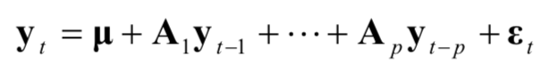
This can be rewritten as:
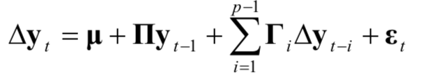
where:
In the second equation above we have multidimensional variables and multiplication would happen via matrix multiplication.
The Johansen tests consists of two tests: the maximum eigenvalue test, and the trace test. For both test statistics we test the null hypothesis of no cointegration against the alternative of cointegration, by means of comparing the test statistics to the critical values for the test.
Running the tests
In this section we carry out the mentioned tests and have a closer look at the results of these tests.
Engle Granger and CRDW
Both series (natural logarithms of S2F and bitcoins price) are clearly not stationary, but trending over time. After differencing the series, we might find stationarity for both though.
By the naked eye I would say there is a very good chance that the differenced series are both stationary, but we need to check that as well.
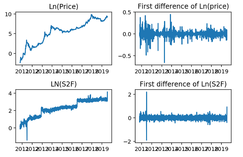
To verify whether the differenced series are stationary I ran the augmented Dickey-Fuller (ADF) test for both differenced series. Code for the test is in the appendix.
ADF test result for first order difference of ln(price)
ADF Statistic: -12.843153
p-value: 0.000000
Critical Values:
	1%: -3.432
	5%: -2.862
	10%: -2.567
ADF test result for first order difference of ln(S2F)
ADF Statistic: -15.426991
p-value: 0.000000
Critical Values:
1%: -3.432
5%: -2.862
10%: -2.567For both series we can reject the null hypothesis of the presence of a unit root, which tells us we can say with at least 99% certainty that both variables are not integrated of the first order. Time to run an OLS regression to estimate the coefficients in:
lnBTCprice_𝑡 =α+𝛽 lnS2F_𝑡+e_𝑡
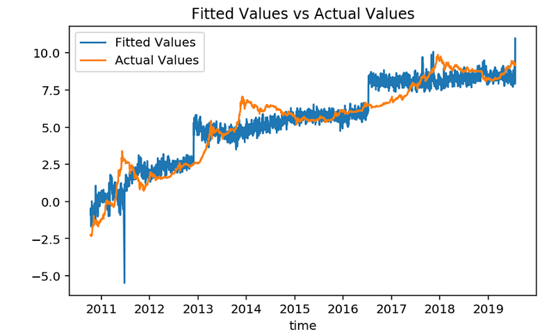
Here’s the regression summary which we use for both CRDW and the Engle and Granger procedure.
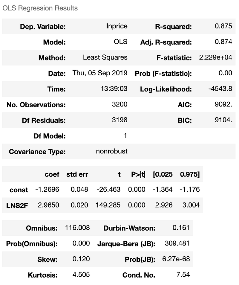
We’ll have a closer look at the residuals from that regression. The residuals as shown below don’t look like a stationary series, but the Durbin Watson statistic is just significantly larger than zero for~3200 observations, so even though the residual plot indicates no cointegration, the CRDW test statistic (value=0.161) doesn’t support this!
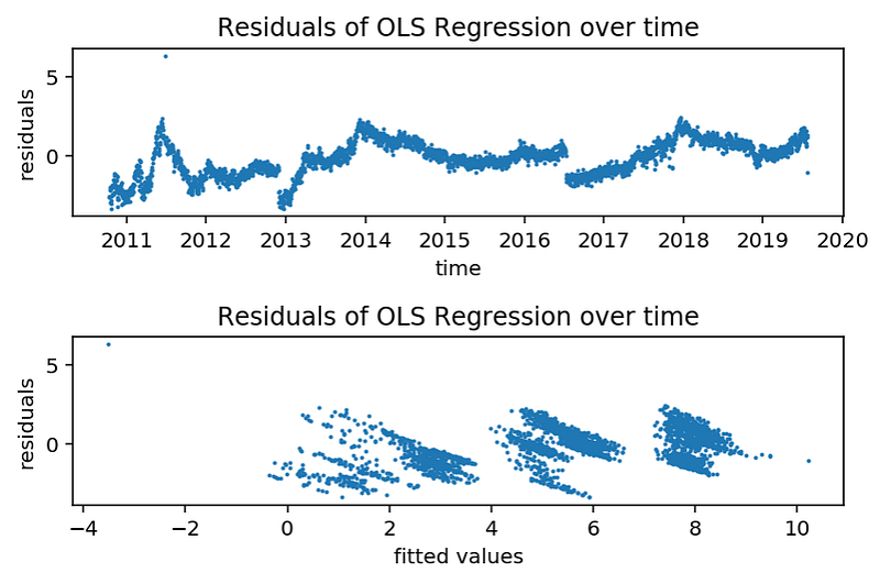
I ran the ADF test to check for unit root in the residuals. According to the ADF test we have to reject the null hypothesis and conclude that the residuals are stationary. The concept of cointegration is again not rejected!
ADF test result for regression residuals
ADF Statistic: -3.714701
p-value: 0.003911
Critical Values:
	1%: -3.432
	5%: -2.862
	10%: -2.567
Johansen test
As mentioned the Johansen test consists of two separate tests; the maximum eigenvalue test and the trace test. The statsmodels package in Python was used to conduct the tests. Code can be found in the Appendix.
Trace Statistic:
[77.61330689  8.83704667]
Critical Values Trace Statistic [90% 95% 99%]:
[[13.4294 15.4943 19.9349]
 [ 2.7055  3.8415  6.6349]]
Maximum Eigenvalue Statistic
[68.77626022  8.83704667]
Critical Values Maximum Eigenvalue Statistic [90% 95% 99%]
[[12.2971 14.2639 18.52  ]
 [ 2.7055  3.8415  6.6349]]
For both Johansen tests we fail to reject the null hypothesis (as the test statistics are higher than critical values for all confidence intervals).
Conclusion
The estimated relation between lnBTCprice and lnS2F is consistent (even though the OLS assumptions are not met) as we have shown that the time series are cointegrated. My former conclusion is thereby falsified. As cointegration applies we are able to use the coefficients coming from the OLS to quantify a model that describes the relation between the two series.
[UPDATE] This conclusion will be proven wrong in a follow up article.
We could set up a Vector Error Correction Model to model both the short term and the long term dynamics of the relation, which I leave for a follow up article.
References
[1]:https://readmedium.com/modeling-bitcoins-value-with-scarcity-91fa0fc03e25
[3]: https://readmedium.com/falsifying-stock-to-flow-as-a-model-of-bitcoin-value-b2d9e61f68af
[4]: Co-Integration and Error Correction: Representation, Estimation, and Testing; Robert F. Engle and C. W. J. Granger, 1987
[5]: A guide to Modern Econometrics, second edition, 2005; M. Verbeek
Appendix
Python code
https://gist.github.com/MarcelBurger/ed216b12e436bb4f07497cecff2b6742


