Introduction

Recently Plan B, an early Dutch bitcoin adopter who anonymously shares his insights via Twitter, came out with an article [1] that dives into the relation between bitcoin’s price (and market cap) and the stock-to-flow ratio. It has attracted a lot of attention and the crypto community really praises his analysis. People fell in love with the conclusions that followed from his analysis, which is easy to understand as it predicts future price levels of six figures and more. Even though the idea of investigating market capitalisation or price as a function of stock-to-flow ratio’s is very interesting, one should respect the underlying model assumptions that hold for ordinary least squares regression. In this article I’ll pinpoint the flaws of the analysis, and I’ll have a look at alternative methods to come up with an improved model in a follow up article. I can’t guarantee I can find a model that is statistically significant and respects all the imposed assumptions though.

Respecting the assumptions

Plan B attempted to fit a model that describes the relation between the natural logarithm of bitcoins market cap and the natural logarithm of the stock-to-flow ratio by means of ordinary least squares regression. The standard set of 4 (Gaus-Markov) assumptions that needs to be respected (see Verbeek, Modern Econometrics [2]) are as follows :

- (1) The expected value of the error term is zero (which means that on average the regression should be correct)

- (2) The error and the independent variables should be independent.

- (3) The error term should be homoskedastic (i.e. error terms have the same variance)

- (4) There should be zero correlation between different error terms (i.e. autocorrelation is excluded)

Together, (1), (3) and (4) imply that the error terms are uncorrelated drawings from a distribution with expectation zero and constant variance. If the above assumptions are not met, the standard errors of the coefficients might be biased and therefore the results of the significance tests don’t mean that much anymore. In order to draw conclusions based on the ANOVA results, we also have to check if the underlying model assumptions hold.

A review of plan B’s model

To make sure the review is appropriate, I have used Plan B’s dataset. In my own dataset I’ll introduce some improvements, but for now his dataset is used. After running the exact same regression analysis in which the natural logarithms of the stock-to-flow of bitcoin acts as the independent variable to explain the natural logarithm of the market cap of bitcoin as the dependent variable, I found the same test results.

Checking the assumptions: Autocorrelation

A quick glance at the residual plots (one vs time, the other vs the predicted values), shows that there is some kind of periodic effect observable in the second scatter plot.

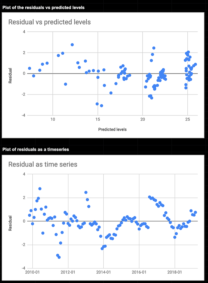
As the second chart clearly shows a certain pattern, we have to test for autocorrelation. Both the Durbin-Watson test and the test for autoregression (by regressing the residual terms on their lagged values in case of first order autocorrelation) show we have to reject the hypothesis that there is no first order autocorrelation in the error terms.

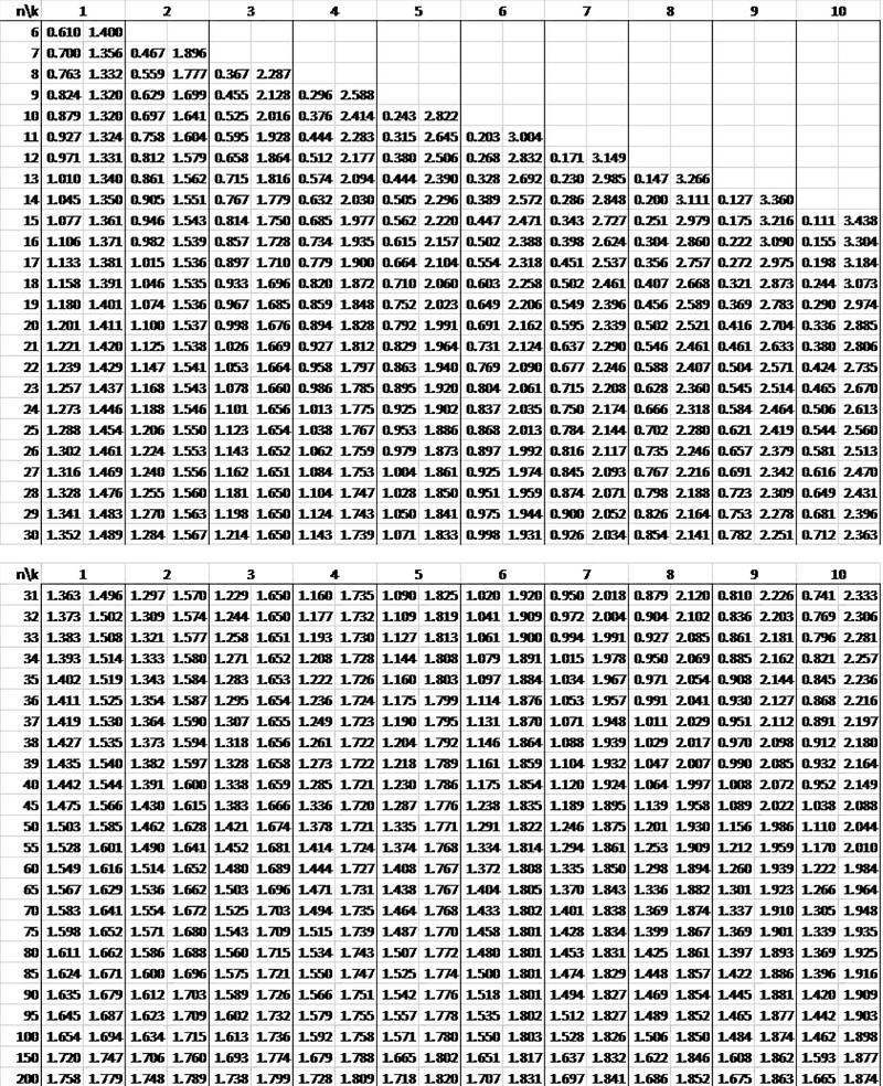
The Durbin Watson statistic turned out to be ~0.4 which was much smaller than the lower bound value of 1.654~1.72 (see the table [4] in the appendix) which we would have to use for our dataset as the 5% lower bound of the critical value. The anova results for the regression test are also shown below.

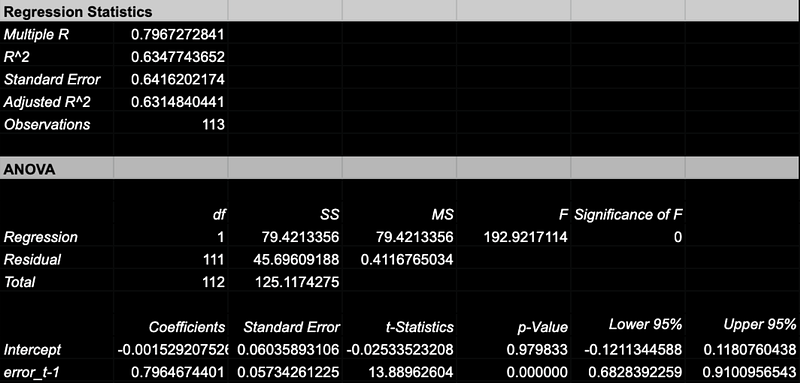
Or in layman terms; we have to find a better model as the significance tests are biased as a result of serial correlation in the residual. The model indicates that the error at time t is a function of 0.796 times the error at time t-1 plus some noise.

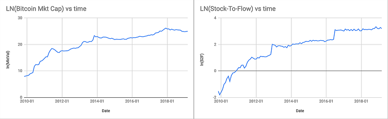
This should not come as a complete surprise as both time series are non-stationary. There is a clear upward trend for both time series as can be seen in the graphs below. One way to deal with this can be found in differencing the time series or in case of asset price evolution looking at the periodic returns instead. This is however not a guarantee that the problem of autocorrelation is solved immediately or that the model returns significant estimators.

EDIT: Econometricians learn to always use returns, log returns or differencing when studying timeseries of asset prices to get rid of non stationarity in the time series. Non-stationary time series in financial models are likely to produce unreliable and spurious results and as a consequence lead to poor understanding and forecasting.

Checking the assumptions: Heteroskedasticity

Aside from checking for autocorrelation, we also have to check for heteroskedasticity. A plot of the squared residuals could show us if we might expect heteroskedasticity.

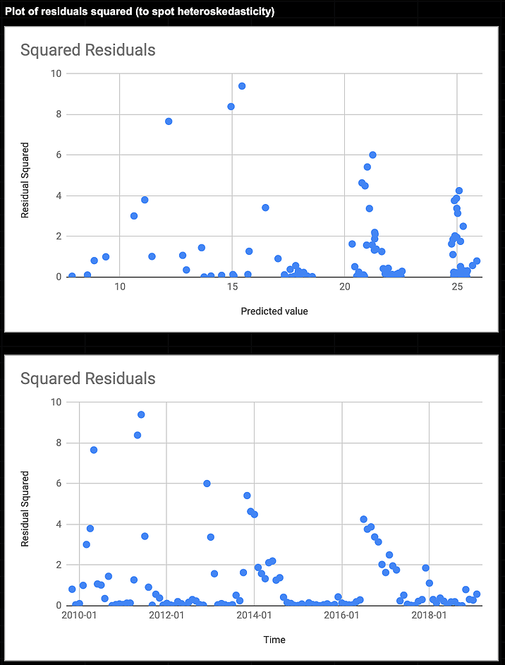
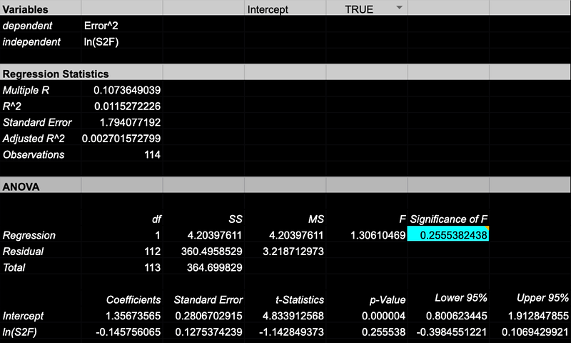
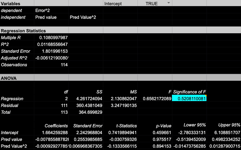
At a first glance it seems like the error doesn’t have the same variance everywhere, which would imply heteroskedasticity. In order to confirm the suspicions, I ran both the Whites test and the Breusch-Pagan test. In both cases we have to reject the null-hypothesis of heteroskedasticity being present in the model. In laymen terms; we are not able to state that the model suffers from heteroskedasticity, which is good! Test results for Whites and Breusch-Pagan are below.

Minor data issue

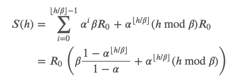
I have downloaded the data used by Plan B from his github repository to replicate and review his work. I noticed there was a little error in the number of bitcoins created over time. In his data set he did not change mining rewards every 210.000 blocks (as follows from the protocol) but instead he shifted to a new mining reward regime once the monthly measured block height passed another 210.000 blocks. I expect the resulting error to be not really significant, but decided to use a closed form formula that exactly returns the number of bitcoins into existence as a function of block height. The function follows from solving the initial value problem for the differential equation that describes the growth of the bitcoin supply. This is perfectly explained by Onur Solmaz [3] in his article on the bitcoin inflation curvature. In this function the following variables are defined:

- S: the total supply

- R0: the initial mining reward = 50

- alpha: the reward decay factor = 0.5

- h: blockheight

- beta: the milestone number of blocks before a decrease of the reward kicks in = 210.000

Please note that the floor function is used where h is divided by beta.

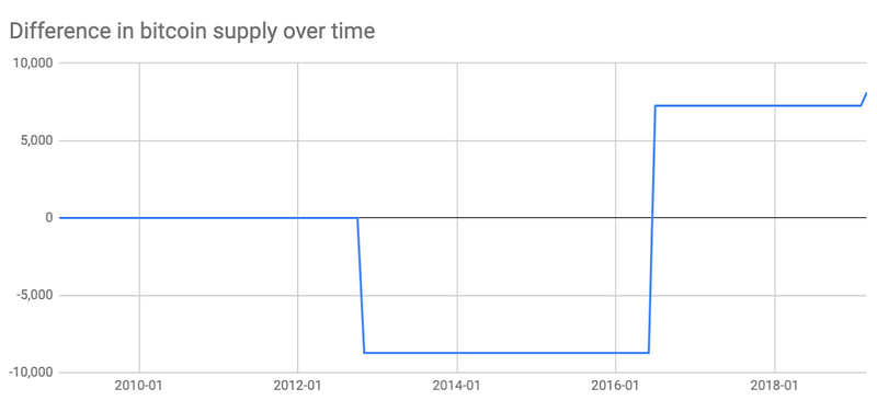
The graph below shows how the number of bitcoins over time in Plan B’s dataset differ from the true supply.

Conclusion

With the model suffering from autocorrelation in the residuals, we have to reject the current model and come up with a better model. For most quants it is nothing new that explanatory models w.r.t. asset performance are always using returns or log returns to avoid autocorrelation ruining the model. In a follow up article I will check different approaches to help us find a model that meets the assumptions. Unfortunately I can’t guarantee there will be a model that will meet the requirements and will be significant at the same time, but the quant in me is thirsty for improvements to the work that got so much attention from the community.

References

1) https://readmedium.com/modeling-bitcoins-value-with-scarcity-91fa0fc03e25

2) M. Verbeek, A Guide To Modern Econometrics

3) https://solmaz.io/2019/02/09/inflation-curvature-bitcoin-supply/

4) http://www.real-statistics.com/statistics-tables/durbin-watson-table/

Appendix

Durbin Watson Table