Recurrent Neural Networks (RNN) Tutorial — Analyzing Sequential Data Using TensorFlow In Python

In this article, let us discuss the concepts behind the working of Recurrent Neural Networks. Recurrent Neural Networks have wide applications in image and video recognition, music composition and machine translation.

We will be checking out the following concepts:

• Why Not Feed-forward Networks?
• What Are Recurrent Neural Networks?
• How To Train Recurrent Neural Networks?
• Vanishing And Exploding Gradients
• Long Short Term Memory (LSTM) Networks
• LSTM Use-Case

Why Not Feedforward Networks?

Consider an image classification use-case where you have trained the neural network to classify images of various animals.

So, let’s say you feed in an image of a cat or a dog, the network actually provides an output with a corresponding label to the image of a cat or a dog respectively.

Consider the following diagram:

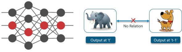
Here, the first output being an elephant will have no influence of the previous output which was a dog. This means that output at time ‘t’ is independent of output at time ‘t-1’.

Consider this scenario where you will require the use of the previously obtained output:

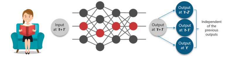
The concept is similar to reading a book. With every page you move forward into, you need the understanding of the previous pages to make complete sense of the information ahead in most of the cases.

With a feed-forward network the new output at time ‘t+1’ has no relation with outputs at either time t, t-1 or t-2.

So, feed-forward networks cannot be used when predicting a word in a sentence as it will have no absolute relation with the previous set of words.

But, with Recurrent Neural Networks, this challenge can be overcome.

Consider the following diagram:

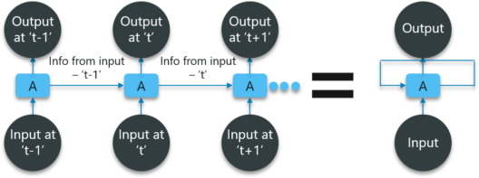
In the above diagram, we have certain inputs at ‘t-1’ which is fed into the network. These inputs will lead to corresponding outputs at time ‘t-1’ as well.

At the next timestamp, information from the previous input ‘t-1’ is provided along with the input at ‘t’ to eventually provide the output at ‘t’ as well.

This process repeats, to ensure that the latest inputs are aware and can use the information from the previous timestamp is obtained.

Next up in this Recurrent Neural Networks article, we need to check out what Recurrent Neural Networks (RNNs) actually are.

What Are Recurrent Neural Networks?

Recurrent Networks are a type of artificial neural network designed to recognize patterns in sequences of data, such as text, genomes, handwriting, the spoken word, numerical times series data emanating from sensors, stock markets and government agencies.

For better clarity, consider the following analogy:

You go to the gym regularly and the trainer has given you the following schedule for your workout:

Note that all these exercises are repeated in a proper order every week. First, let us use a feed-forward network to try and predict the type of exercise.

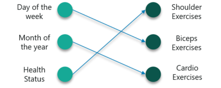
The inputs are day, month, and health status. A neural network has to be trained using these inputs to provide us

with the prediction of the exercises.

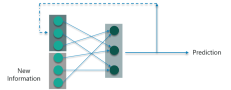
However, this will not be very accurate considering the input. To fix this, we can make use of the concept of Recurrent Neural Networks as shown below:

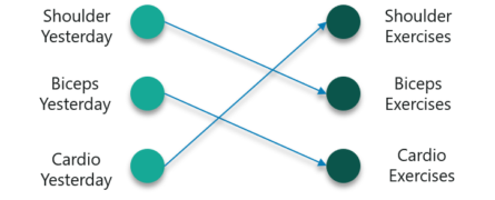
In this case, consider the inputs to be the workout done on the previous day.

So if you did a shoulder workout yesterday, you can do a bicep exercise today and this goes on for the rest of the week as well.

However, if you happen to miss a day at the gym, the data from the previously attended timestamp can be considered as shown below:

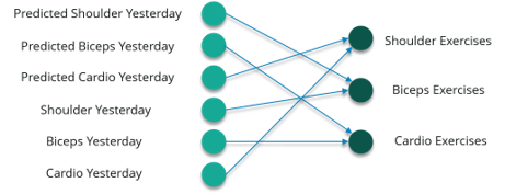
If a model is trained based on the data it can obtain from the previous exercises, the output from the model will be extremely accurate.

To sum it up, let us convert the data we have into vectors. Well, what are vectors?

Vectors are numbers which are input to the model to denote if you have done the exercise or not.

So, if you have a shoulder exercise, the corresponding node will be ‘1’ and the rest of the exercise nodes will be mapped to ‘0’.

Let us check out the math behind the working of the neural network. Consider the following diagram:

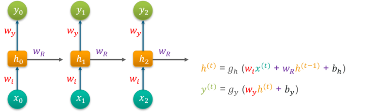
Consider ‘w’ to be the weight matrix and ‘b’ being the bias:

At time t=0, input is ‘x0’ and the task is to figure out what is ‘h0’. Substituting t=0 in the equation and obtaining the function h(t) value. Next, the value of ‘y0’ is found out using the previously calculated values when applied to the new formula.

This process is repeated through all of the timestamps in the model to train a model.

So, how are Recurrent Neural Networks trained?

Training Recurrent Neural Networks

Recurrent Neural Networks use a backpropagation algorithm for training, but it is applied for every timestamp. It is commonly known as Back-propagation Through Time (BTT).

There are some issues with Back-propagation such as:

• Vanishing Gradient
• Exploding Gradient

Let us consider each of these to understand what is going on

Vanishing Gradient

When making use of back-propagation the goal is to calculate the error which is actually found out by finding out the difference between the actual output and the model output and raising that to a power of 2.

Consider the following diagram:

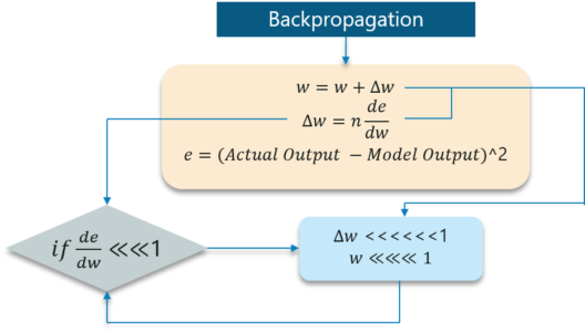
With the error calculated, the changes in the error with respect to the change in the weight is calculated. But with each learning rate, this has to be multiplied with the same.

So, the product of the learning rate with the change leads to the value which is the actual change in the weight.

This change in weight is added to the old set of weights for every training iteration as shown in the figure. The issue here is when the change in weight is multiplied, the value is very less.

Consider you are predicting a sentence say,“I am going to France” and you want to predict “I am going to France, the language spoken there is _____”

A lot of iterations will cause the new weights to be extremely negligible and this leads to the weights not being updated.

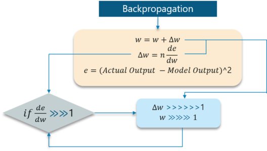
Exploding Gradient

The working of the exploding gradient is similar but the weights here change drastically instead of negligible change. Notice the small change in the diagram below:

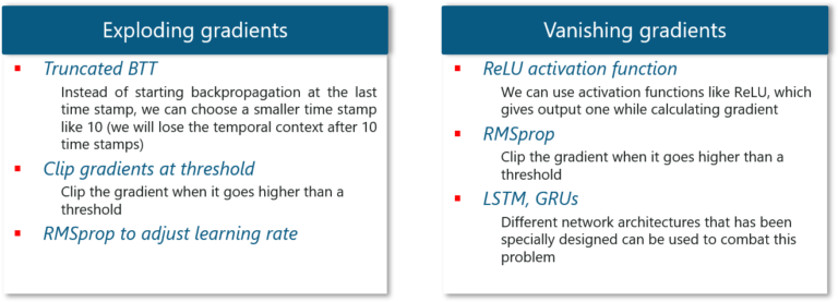
We need to overcome both of these and it is a bit of a challenge at first. Consider the following chart:

Continuing this blog on Recurrent Neural Networks, we will be discussing further on LSTM networks.

Long Short-Term Memory Networks

Long Short-Term Memory networks are usually just called “LSTMs”.

They are a special kind of Recurrent Neural Networks that are capable of learning long-term dependencies.

What are long-term dependencies?

Many times only recent data is needed in a model to perform operations. But there might be a requirement from data which was obtained in the past.

Let’s look at the following example:

Consider a language model trying to predict the next word based on the previous ones. If we are trying to predict the last word in the sentence say “The clouds are in the sky”.

The context here was pretty simple and the last word ends up being sky all the time. In such cases, the gap between the past information and the current requirement can be bridged really easily by using Recurrent Neural Networks.

So, problems like Vanishing and Exploding Gradients do not exist and this makes LSTM networks handle long-term dependencies easily.

LSTM has a chain-like neural network layer. In a standard recurrent neural network, the repeating module consists of one single function as shown in the below figure:

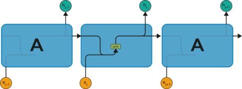
As shown above, there is a tanh function present in the layer. This function is a squashing function. So, what is a squashing function?

It is a function which is basically used in the range of -1 to +1 and to manipulate the values based on the inputs.

Now, let us consider the structure of an LSTM network:

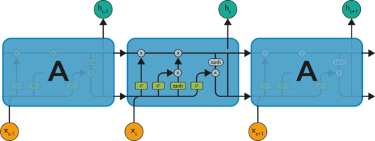
As denoted from the image, each of the functions in the layers has their own structures when it comes to LSTM networks. The cell state is the horizontal line in the figure and it acts like a conveyer belt carrying certain data linearly across the data channel.

Let us consider a step-by-step approach to understand LSTM networks better.

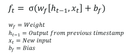
Step 1:

The first step in the LSTM is to identify that information which is not required and will be thrown away from the cell state. This decision is made by a sigmoid layer called as forget gate layer.

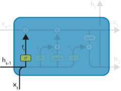
The highlighted layer in the above is the sigmoid layer which is previously mentioned.

The calculation is done by considering the new input and the previous timestamp which eventually leads to the output of a number between 0 and 1 for each number in that cell state.

As typical binary, 1 represents to keep the cell state while 0 represents to trash it.

Consider gender classification, it is really important to consider the latest and correct gender when the network is being used.

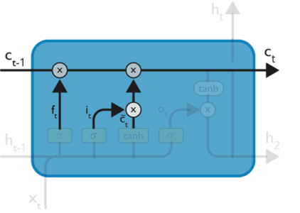
Step 2:

The next step is to decide, what new information we’re going to store in the cell state. This whole process comprises of following steps:

• A sigmoid layer called the “input gate layer” decides which values will be updated.
• The tanh layer creates a vector of new candidate values, that could be added to the state.

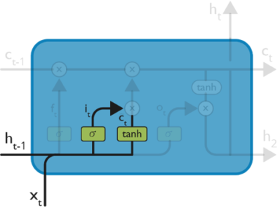
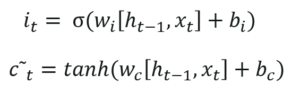
The input from the previous timestamp and the new input are passed through a sigmoid function which gives the value i(t). This value is then multiplied by c(t) and then added to the cell state.

In the next step, these two are combined to update the state.

Step 3:

Now, we will update the old cell state Ct−1, into the new cell state Ct.

First, we multiply the old state (Ct−1) by f(t), forgetting the things we decided to leave behind earlier.

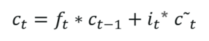
Then, we add i_t* c˜_t. This is the new candidate values, scaled by how much we decided to update each state value.

In the second step, we decided to do make use of the data which is only required at that stage.

In the third step, we actually implement it.

In the language case example which was previously discussed, there is where the old gender would be dropped and the new gender would be considered.

Step 4:

We will run a sigmoid layer which decides what parts of the cell state we’re going to output.

Then, we put the cell state through tanh (push the values to be between −1 and 1)

Later, we multiply it by the output of the sigmoid gate, so that we only output the parts we decided to.

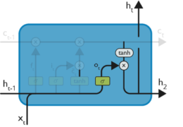
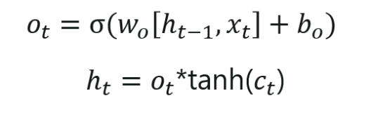
The calculation in this step is pretty much straightforward which eventually leads to the output.

However, the output consists of only the outputs there were decided to be carry forwarded in the previous steps and not all the outputs at once.

Summing up all the 4 steps:

In the first step, we found out what was needed to be dropped.

The second step consisted of what new inputs are added to the network.

The third step was to combine the previously obtained inputs to generate the new cell states.

Lastly, we arrived at the output as per requirement.

Next up, let us consider an interesting use-case.

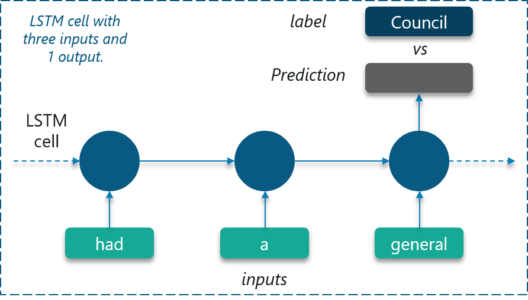
Use Case: Long Short-Term Memory Networks

The use case we will be considering is to predict the next word in a sample short story.

We can start by feeding an LSTM Network with correct sequences from the text of 3 symbols as inputs and 1 labeled symbol.

Eventually, the neural network will learn to predict the next symbol correctly!

Dataset:

The LSTM is trained using a sample short story which consists of 112 unique symbols. Comma and period are also considered as unique symbols in this case.

“long ago, the mice had a general council to consider what measures they could take to outwit their common enemy, the cat . some said this, and some said that but at last a young mouse got up and said he had a proposal to make, which he thought would meet the case . you will all agree , said he , that our chief danger consists in the sly and treacherous manner in which the enemy approaches us . now, if we could receive some signal of her approach, we could easily escape from her . i venture, therefore, to propose that a small bell be procured, and attached by a ribbon round the neck of the cat. by this means we should always know when she was about, and could easily retire while she was in the neighborhood. this proposal met with general applause until an old mouse got up and said that is all very well, but who is to bell the cat? the mice looked at one another and nobody spoke. then the old mouse said it is easy to propose impossible remedies .”

Training:

We already know that LSTMs can only understand real numbers. So, the first requirement is to convert the unique symbols into unique integer values based on the frequency of occurrence.

Doing this will create a customized dictionary that we can make use of later on to map the values.

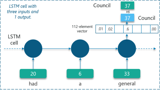
In the above figure, certain symbols are mapped to be integers as shown.

The network will create a 112-element vector consisting of the probability of occurrence of each of these unique integer values.

Implementation:

The code is implemented using Tensorflow as shown below:

import numpy as np
import tensorflow as tf
from tensorflow.contrib import rnn
import random
import collections
import time
 
start_time = time.time()
 
def elapsed(sec):
    if sec<60:
        return str(sec) + " sec"
    elif sec<(60*60): return str(sec/60) + " min" else: return str(sec/(60*60)) + " hr" # Target log path logs_path = '/tmp/tensorflow/rnn_words' writer = tf.summary.FileWriter(logs_path) 
# Text file containing words for training training_file = 'Story.txt' def read_data(fname): with open(fname) as f: content = f.readlines() content = [x.strip() for x in content] content = [content[i].split() for i in range(len(content))] content = np.array(content) content = np.reshape(content, [-1, ]) return content training_data = read_data(training_file) print("Loaded training data...") def build_dataset(words): count = collections.Counter(words).most_common() dictionary = dict() for word, _ in count: dictionary[word] = len(dictionary) reverse_dictionary = dict(zip(dictionary.values(), dictionary.keys())) return dictionary, reverse_dictionary dictionary, reverse_dictionary = build_dataset(training_data) vocab_size = len(dictionary) 
# Parameters learning_rate = 0.001 training_iters = 50000 display_step = 1000 n_input = 3 
# number of units in RNN cell n_hidden = 512 
# tf Graph input x = tf.placeholder("float", [None, n_input, 1]) y = tf.placeholder("float", [None, vocab_size]) 
# RNN output node weights and biases weights = { 'out': tf.Variable(tf.random_normal([n_hidden, vocab_size])) } biases = { 'out': tf.Variable(tf.random_normal([vocab_size])) } def RNN(x, weights, biases): 
# reshape to [1, n_input] x = tf.reshape(x, [-1, n_input])
# Generate a n_input-element sequence of inputs 
# (eg. [had] [a] [general] -> [20] [6] [33])
    x = tf.split(x,n_input,1)
 
    # 2-layer LSTM, each layer has n_hidden units.
    # Average Accuracy= 95.20% at 50k iter
    rnn_cell = rnn.MultiRNNCell([rnn.BasicLSTMCell(n_hidden),rnn.BasicLSTMCell(n_hidden)])
 
    # 1-layer LSTM with n_hidden units but with lower accuracy.
    # Average Accuracy= 90.60% 50k iter
    # Uncomment line below to test but comment out the 2-layer rnn.MultiRNNCell above
    # rnn_cell = rnn.BasicLSTMCell(n_hidden)
 
    # generate prediction
    outputs, states = rnn.static_rnn(rnn_cell, x, dtype=tf.float32)
 
    # there are n_input outputs but
    # we only want the last output
    return tf.matmul(outputs[-1], weights['out']) + biases['out']
 
pred = RNN(x, weights, biases)
 
# Loss and optimizer
cost = tf.reduce_mean(tf.nn.softmax_cross_entropy_with_logits(logits=pred, labels=y))
optimizer = tf.train.RMSPropOptimizer(learning_rate=learning_rate).minimize(cost)
 
# Model evaluation
correct_pred = tf.equal(tf.argmax(pred,1), tf.argmax(y,1))
accuracy = tf.reduce_mean(tf.cast(correct_pred, tf.float32))
 
# Initializing the variables
init = tf.global_variables_initializer()
 
# Launch the graph
with tf.Session() as session:
    session.run(init)
    step = 0
    offset = random.randint(0,n_input+1)
    end_offset = n_input + 1
    acc_total = 0
    loss_total = 0
 
    writer.add_graph(session.graph)
 
    while step < training_iters: # Generate a minibatch. Add some randomness on selection process. if offset > (len(training_data)-end_offset):
            offset = random.randint(0, n_input+1)
 
        symbols_in_keys = [ [dictionary[ str(training_data[i])]] for i in range(offset, offset+n_input) ]
        symbols_in_keys = np.reshape(np.array(symbols_in_keys), [-1, n_input, 1])
 
        symbols_out_onehot = np.zeros([vocab_size], dtype=float)
        symbols_out_onehot[dictionary[str(training_data[offset+n_input])]] = 1.0
        symbols_out_onehot = np.reshape(symbols_out_onehot,[1,-1])
 
        _, acc, loss, onehot_pred = session.run([optimizer, accuracy, cost, pred], \
                                                feed_dict={x: symbols_in_keys, y: symbols_out_onehot})
        loss_total += loss
        acc_total += acc
        if (step+1) % display_step == 0:
            print("Iter= " + str(step+1) + ", Average Loss= " + \
                  "{:.6f}".format(loss_total/display_step) + ", Average Accuracy= " + \
                  "{:.2f}%".format(100*acc_total/display_step))
            acc_total = 0
            loss_total = 0
            symbols_in = [training_data[i] for i in range(offset, offset + n_input)]
            symbols_out = training_data[offset + n_input]
            symbols_out_pred = reverse_dictionary[int(tf.argmax(onehot_pred, 1).eval())]
            print("%s - [%s] vs [%s]" % (symbols_in,symbols_out,symbols_out_pred))
        step += 1
        offset += (n_input+1)
    print("Optimization Finished!")
    print("Elapsed time: ", elapsed(time.time() - start_time))
    print("Run on command line.")
    print("\ttensorboard --logdir=%s" % (logs_path))
    print("Point your web browser to: http://localhost:6006/")
    while True:
        prompt = "%s words: " % n_input
        sentence = input(prompt)
        sentence = sentence.strip()
        words = sentence.split(' ')
        if len(words) != n_input:
            continue
        try:
            symbols_in_keys = [dictionary[str(words[i])] for i in range(len(words))]
            for i in range(32):
                keys = np.reshape(np.array(symbols_in_keys), [-1, n_input, 1])
                onehot_pred = session.run(pred, feed_dict={x: keys})
                onehot_pred_index = int(tf.argmax(onehot_pred, 1).eval())
                sentence = "%s %s" % (sentence,reverse_dictionary[onehot_pred_index])
                symbols_in_keys = symbols_in_keys[1:]
                symbols_in_keys.append(onehot_pred_index)
            print(sentence)
        except:
            print("Word not in dictionary")

This brings us to the end of our article on “Recurrent Neural Networks”. I hope you found this article informative and added value to your knowledge.

If you wish to check out more articles on the market’s most trending technologies like Artificial Intelligence, DevOps, Ethical Hacking, then you can refer to Edureka’s official site.

Do look out for other articles in this series which will explain the various other aspects of Deep Learning.

1. TensorFlow Tutorial

2. PyTorch Tutorial

3. Perceptron learning Algorithm

4. Neural Network Tutorial

5. What is Backpropagation?

6. Convolutional Neural Networks

7. Capsule Neural Networks

8. Object Detection in TensorFlow

9. Autoencoders Tutorial

10. Restricted Boltzmann Machine Tutorial

11. PyTorch vs TensorFlow

12. Deep Learning With Python

13. Artificial Intelligence Tutorial

14. TensorFlow Image Classification

15. Artificial Intelligence Applications

16. How to Become an Artificial Intelligence Engineer?

17. Q Learning

18. Apriori Algorithm

19. Markov Chains With Python

20. Artificial Intelligence Algorithms

21. Best Laptops for Machine Learning

22. Top 12 Artificial Intelligence Tools

23. Artificial Intelligence (AI) Interview Questions

24. Theano vs TensorFlow

25. What Is A Neural Network?

26. Pattern Recognition

27. Alpha Beta Pruning in Artificial Intelligence

Originally published at www.edureka.co on November 28, 2018.