
Olympic Medal Numbers Predictions with Time Series, Part 2: Data Analysis
Fbprophet, Darts, AutoTS, Arima, Sarimax and Monte Carlo Simulation

If you didn’t read part 1, here is the link; Part 1. In part 1 we did missing value imputing, constant column droping, finding incorrectly spelt words and fixing incorrectly spelt words.
Data Preparation
In this work we focus on Athletics sport that one of the most popular olympic games. You can see, athletics medal numbers are different by year. Also there are some olympic games played after two year later like 1906. They are important informations but in this problem, they will not much effect on forecasting models.
df_athletics = data_clean[data_clean['Sport'] == 'Athletics']
df_athletics['Medal_Num'] = 1
df_athletics_timeseries = df_athletics.groupby(['Year']).sum()
print(df_athletics_timeseries.head())
print(df_athletics_timeseries.tail())
Medal_Num
Year
1896 37
1900 76
1904 79
1906 65
1908 101
Medal_Num
Year
2000 190
2004 180
2008 187
2012 190
2016 192This is total numbers of medals but we interest about medal numbers of each country. You can see below how calculate total number of medals for each year and each country.
for team in df_athletics['Team'].unique():
    selected_df = df_athletics[df_athletics['Team'] == team]
    temp_group_df = selected_df.groupby(['Year']).sum()
    df_athletics_timeseries[team] = 0
    df_athletics_timeseries.loc[temp_group_df.index, team] = temp_group_df['Medal_Num']
print(df_athletics_timeseries.head())
print(df_athletics_timeseries.tail())
Medal_Num Russia Spain Unified Team Ethiopia Sweden \...
Year
1896 37 0 0 0 0 0
1900 76 0 0 0 0 1
1904 79 0 0 0 0 0
1906 65 0 0 0 0 11
1908 101 0 0 0 0 5 Medal_Num Russia Spain Unified Team Ethiopia Sweden \...
Year
2000 190 18 1 0 8 1
2004 180 27 3 0 7 3
2008 187 25 0 0 7 0
2012 190 23 0 0 7 0
2016 192 0 2 0 8 0 Data Analysis
There are 103 country in dataset. When analyzing data, we are just focus on United States that has most numbers medal of athletics games in olympics.
We plot the rolling mean for seeing the trends of data. There is a big gap in 1980. When we are searching about that, we realize United State led a boycott of the Summer Olympic Games in 1980. You can read more from this link https://2001-2009.state.gov/r/pa/ho/time/qfp/104481.htm. Actually this is a missing value but now we forget about this.
df_athletics_timeseries_US = df_athletics_timeseries['United States'].copy()g = sns.lineplot(x=df_athletics_timeseries_US.index, y=df_athletics_timeseries_US, label="Actual Time Series")
rmean = df_athletics_timeseries_US.rolling(4, win_type='triang').mean()
g = sns.lineplot(x=rmean.index, y=rmean, label="Rolling Mean 4")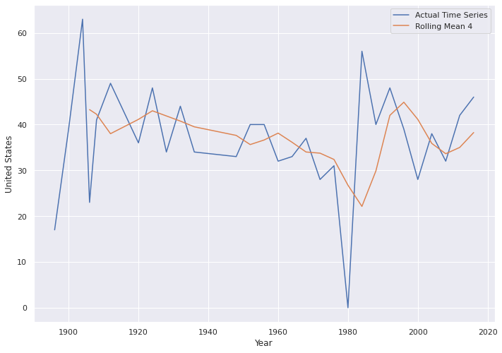
Now we check the data is okay for forecasting by looking p-values. We use auto_arima for finding the best order and statsmodels sarimax for data analysis. P-value should be low for better forecasting. In our problem 0.542 is not good but it doesn’t mean this data can not be forecastable. You will see our forecasting models have better perform than mean model (random model).
The distribution of data is normal distribution. It makes forecasting easier. We can understand it from q-q plot and histogram plot.
from pmdarima import auto_arima

stepwise_fit = auto_arima(df_athletics_timeseries_US, trace=False, suppress_warning=True)
mod = sm.tsa.statespace.SARIMAX(df_athletics_timeseries_US,
                                order=stepwise_fit.order,
                                seasonal_order=(1, 1, 1, 4),
                                enforce_stationarity=False,
                                enforce_invertibility=False)

results = mod.fit()

print(results.summary().tables[1])
====================================================================
coef std err z P>|z|
------------------------------------------------------------------------------
ar.S.L4 -0.1904 0.351 -0.542 0.588
ma.S.L4 -1.0000 8615.494 -0.000 1.000
sigma2 110.9240 9.56e+05 0.000 1.000
====================================================================results.plot_diagnostics(figsize=(16, 8))
plt.show()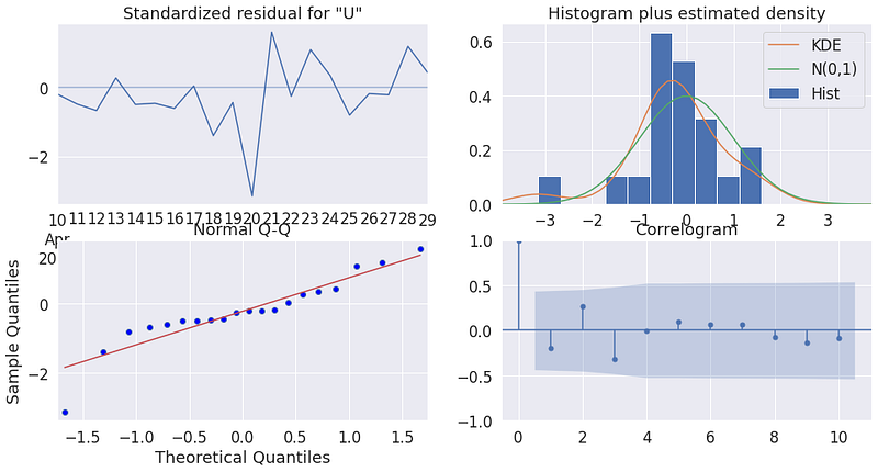
Future Medal Numbers Forecasting
Then we try to the forecast next medal numbers by using one-step-ahead forecast. It gives us information about can data predictable. This forecasting is still a part of data analysis.
Time series models need time series index but olympic dataset has just years. Because of we rescale time to start 2021–04–01 and end 2021–04–29.
pred = results.get_prediction(
    start=pd.to_datetime('2021-04-26'), dynamic=False)

ax = df_athletics_timeseries_US.plot(label='observed')
pred.predicted_mean.plot(ax=ax, label='One-step ahead Forecast', alpha=.8, figsize=(14, 7))

ax.set_xlabel('index')
ax.set_ylabel('Real Total Medals US')

plt.legend()
plt.show()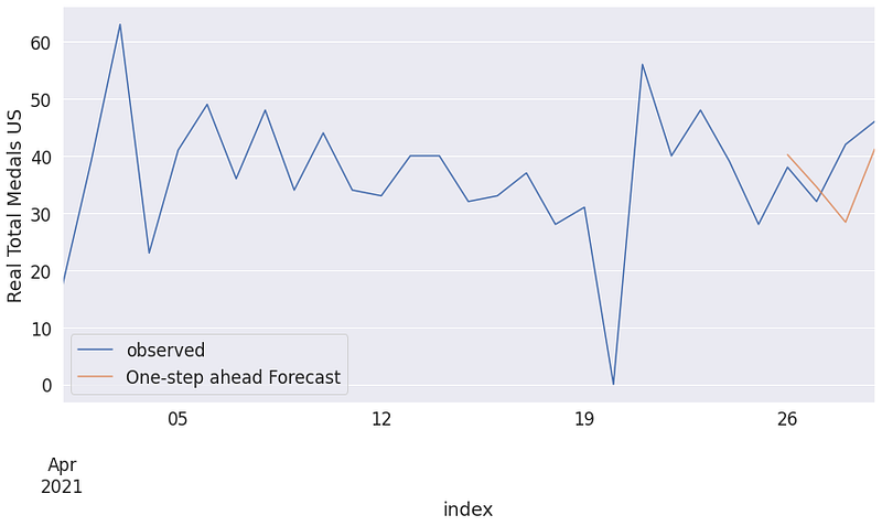
pred_uc = results.get_forecast(steps=10)
pred_ci = pred_uc.conf_int()

ax = df_athletics_timeseries_US.plot(label='Total Medals US', figsize=(14, 7))

pred_uc.predicted_mean.plot(ax=ax, label='Forecast')

ax.fill_between(pred_ci.index,
                pred_ci.iloc[:, 0],
                pred_ci.iloc[:, 1], color='k', alpha=.15)

ax.set_xlabel('index')
ax.set_ylabel('Real Total Medals US')

plt.legend()
plt.show()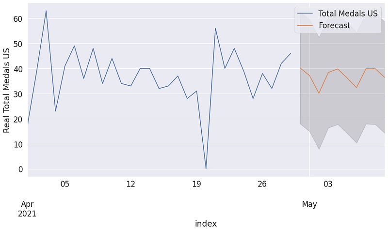
These graph show us the sarimax model can understand some pattern that is inside the dataset but one model can can mislead us. So we should select another model for better understand dataset. In this problem, we choose fbprophet that is good time series model especially for seasonal dataset. Fbprophet input should have ‘ds’ and ‘y’ columns. Firstly we should prepare data for fbprophet. Then we can fit our time series model.
from fbprophet import Prophet

df_prophet = pd.DataFrame()
df_prophet['y'] = df_athletics_timeseries_US
df_prophet['ds'] = df_athletics_timeseries_US.index

model = Prophet()
model.fit(df_prophet)
For forecasting fbprophet has make_future_dataframe functions. It makes forecasting easier for a data scientist.
Forecasting data has four useful columns. They are ds, yhat, yhat_lower and yhat_upper. ds column is date for the predictions, yhat column is value of predictions, yhat_lower column and yhat_upper are gap for the predictions also they can set manuely.
future = model.make_future_dataframe(periods=10, freq='d')
forecast = model.predict(future)

forecast[['ds', 'yhat', 'yhat_lower', 'yhat_upper']].head()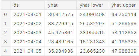
Now we plot the result with plot function that belong to fbprophet. Add_changepoints_to_plot is show us the critical changes in the plot. This prediction has not critical changes but this function is very useful for time series prediction plots.
from fbprophet.plot import add_changepoints_to_plot

fig = model.plot(forecast)

add_changepoints_to_plot(fig.gca(), model, forecast)

plt.show()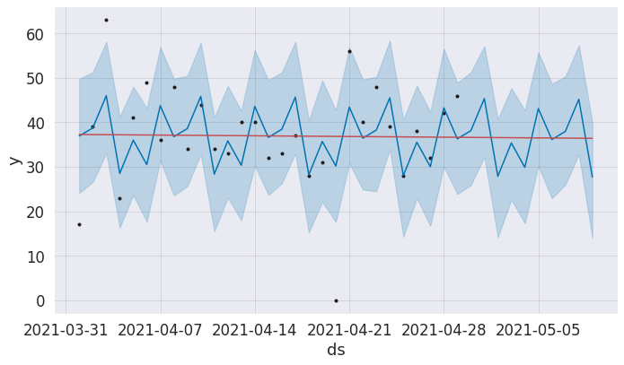
Discussion and Conclusions
Data looks predictable and not random. P-value is not what we expected but it can be better with more data cleaning. For example, in 1980, 65 nations refused to participate in the games, whereas 80 countries sent athletes to compete. This is bad for forecasting problems and it can fix for more successful time series models.
👋 Thanks for reading. If you enjoy my work, don’t forget to like, follow me on medium and on LinkedIn. It will motivate me in offering more content to the Medium community ! 😊

Data analysis part ends here. You can keep reading about forecasting in part 3. The link is Part 3. In part 3 we used eleven-time series model. They are six main model, four sub-model and one mean prediction (Fbprophet, Darts, AutoTS, Arima, Sarimax and Monte Carlo Simulation).
References:
[1]: https://www.kaggle.com/heesoo37/120-years-of-olympic-history-athletes-and-results [2]: https://www.kaggle.com/hasanbasriakcay/which-country-is-good-at-which-sports-in-olympics [3]: https://www.kaggle.com/hasanbasriakcay/which-country-is-good-at-which-sports-in-olympics [4]: https://2001-2009.state.gov/r/pa/ho/time/qfp/104481.htm
For More:
Follow DataBulls!


