Nuclear Magnetic Resonance spectroscopy, the overlooked powerhouse of biology -Chapter 2

It’s not all AlphaFold, Cryo-electron microscopy and X-ray diffraction of crystals when it comes to studying the atomic structure of biological matter. The much-overlooked technique of nuclear magnetic resonance can fill many voids that other techniques can’t even approach. Here we move into NMR’s key concepts, important for the next chapters, and overview what’s coming next regarding applications to biology.

If you are totally new to NMR, check out the introductory chapter first:

As we saw in the first chapter, NMR spectroscopy is different to other spectroscopies in that the main signals arise from individual nuclei, hence atoms. Thus, NMR can provide highly detailed information, yep, right at atomic resolution.

Each NMR resonance or signal has 3 main features that depend, and hence report, on molecular structure and dynamics.

We will next explore these features and how they relate to structure and dynamics at a rather theoretical level that will be the basis for understanding concrete applications later on.

The 3 main features of NMR resonances and how they relate to molecular structure and dynamics

NMR resonances can be ascribed three main global features, from which we can extract information about each specific atom or small sets of atoms in the molecule:

• Chemical shift, or position in the spectrum: Each nucleus, say ¹H, ¹³C, etc. resonates at a small deviation from its “central” frequency, called the Larmor frequency, which is of say around 800 MHz for ¹H in a static magnetic field of around 18.8 T or around 80 MHz for ¹⁵N in the same static magnetic field. The exact value that each resonance deviates from a central frequency is called the “chemical shift”. Different nuclei of the same isotope, such as say the nucleus of an H atom bound to a secondary carbon, or to an aromatic carbon, or to a nitrogen, just to pose three examples, will resonate in slightly different positions of the spectrum, in the order of some units, tens, or hundreds of millionths of the central frequency -the “chemical shift”. Normally we measure this in parts per million from the central frequency, so the units of chemical shift are “ppm”.
• Couplings to other nuclei that are close, either through covalent connectivity or over space: Each nucleus can “feel” the state of nearby nuclei through so-called couplings. This magnetic interaction can take place through covalent bonds, originating the so-called scalar couplings, or through space, originating dipolar couplings. Couplings result in signal splitting and modulation of the relaxation properties, and thus have information about structure and dynamics.
• Relaxation properties, i.e. how an excited nucleus relaxes back to thermal equilibrium: This is manifested through multiple parameters, with T₁ and T2 relaxation rates being the most important ones. Relaxation properties mainly contain information about molecular motions and chemical equilibria; for example, tumbling in solution modulates relaxation, any internal motions of the atoms also contribute to relaxation, and the exchange of atoms between molecules (most often exchangeable Hs) also modulates relaxation.

Chemical shifts

Going a bit more in detail regarding structural information for proteins, chemical shifts reflect atom type and local structure. Here’s for example a ¹H spectrum of a well-folded protein, where I labeled the areas in which the main kinds of ¹H nuclei resonate:

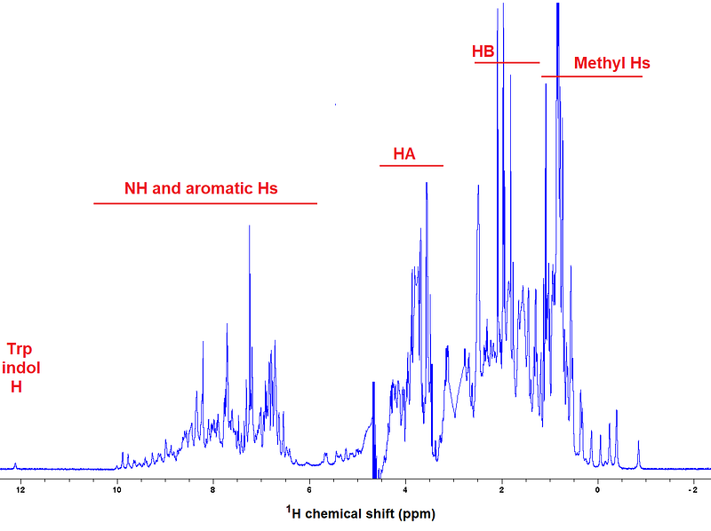
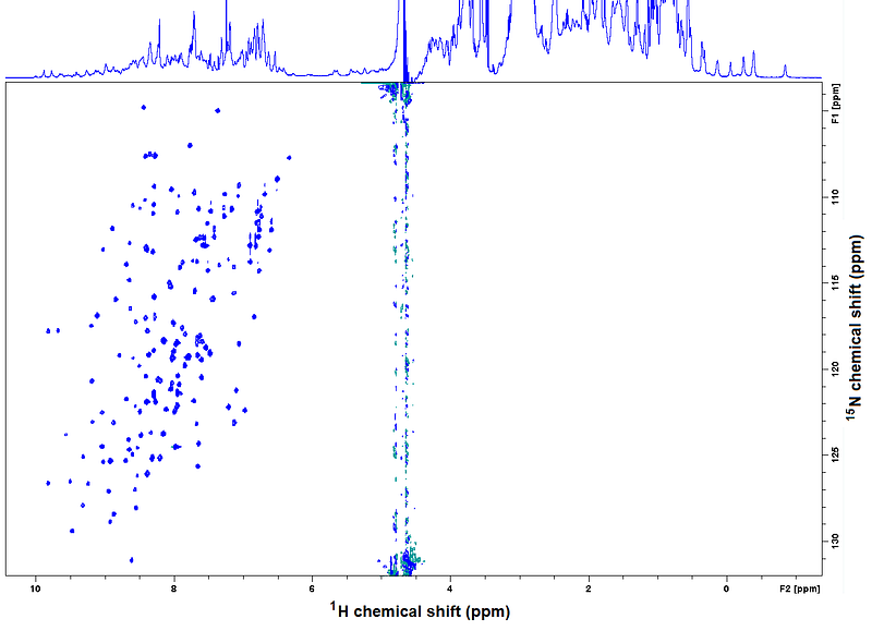
Oh and by the way, a note to connect to the “multidimensional NMR” introduced in Chapter 1 and to advance a very important spectrum for the topics on applications of NMR to proteins, called ¹H-¹⁵N HSQC. Check how the ¹H nuclei from backbone Ns couple to their Ns in a ¹⁵N labeled protein, resulting in a 2D spectrum clean of other correlations:

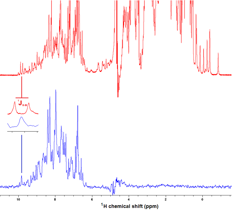
Besides, you can do “exotic” things such as recording a 1D ¹H spectrum selecting signals that arise from H atoms bound to ¹⁵N atoms. This next figure exemplifies this, also showing how the coupling between ¹H and ¹⁵N is collapsed (coupling being another important feature of signals as you’ll see next):

Back to chemical shifts, it is important that in a folded protein the different nuclei of the same type of residue (say all beta carbons of all alanines, for example) resonate in different places, despite being locally equivalent in terms of connectivities to other atoms. This is because in a folded protein the nuclei experience different local environments, an effect that goes extreme in cases of hydrogen bonding, proximity to aromatic rings, etc. Contrary to this, the residues in a highly disordered protein will all feel the same average environment, hence the chemical shifts of nuclei of like residues will all be very similar, close to the “random coil shift”. Somehow, it’s like the residues of a highly disordered protein behave as if they were free amino acids in solution, hence all the same. Instead, residues in a folded protein experience what’s called “chemical shift dispersion”.

One especially important nucleus for structural studies in NMR is ¹³C, because its chemical shifts are very sensitive to local secondary structure. Indeed, if you know the chemical shifts for all backbone + CB resonances of a protein, you can “measure the local secondary structure at each residue”. For this you need to input the ¹³C chemical shifts (plus also ¹H chemical shifts for backbone HN and HA atoms and ¹⁵N shifts for backbone N atoms, which are all typically available) into a program such as “CSI” which calculates the “Chemical Shift Index”, an index that flags each residue as adopting alpha, beta, or coil secondary structure.

Another way to get secondary structure information per residue consists in calculating the so-called “dCA-dCB”, where each dC means the difference between the observed ¹³C (CA or CB) chemical shift and that expected for the corresponding nucleus when the given amino acid is in an unstructured region (the “random coil shift”). The later are tabulated, so the calculation is very easy to compute. As you see, it requires only CA and CB shifts, and it involves a subtraction of subtractions, which means that any calibration errors automatically cancel out. Plus, the result is not just a secondary structure flag per residue but actually a number that varies between say -5 to -2 ppm for a strongly beta-sheet structure to +2-+5 for a strongly helical structure, with numbers between -2 and +2 also having a meaning. Numbers in this range suggest beta sheet or alpha-helical “propensities”, and are widely used to describe the “residual” secondary structure in disordered proteins and in dynamic regions of folded proteins. See for example the analyses I did as part of a work on the intrinsically disordered N-terminal domain of exon 1 in the Huntingtin protein (more specifically, check panel C of Figure 7 here).

Couplings

We saw in the introduction to this chapter that couplings result from the proximity of pairs of NMR-active nuclei in space. This proximity can be mediated directly by covalent bonds, for example between two H atoms bound to the same C atom; or through space, for example between nuclei that belong to residues that are far in a protein’s sequence but get very close in the folded state of the protein. Couplings through bonds are called “scalar” couplings; and couplings through space are called “dipolar” couplings.

In solution, the scalar couplings acting on a signal result in its splitting into duplets, triplets, etc. depending on the pattern of covalent connectivities. You just saw one example in the last figure, where the scalar coupling between a ¹H nucleus and the ¹⁵N nucleus to which it is bound, splits the ¹H’s signal into two components. These components can be brought together back, as you also saw in the example, and most importantly, can be exploited to transfer magnetization between nuclei and generate correlations in multiple dimensions, as you saw two figures ago in the ¹H-¹⁵N HSQC spectrum.

The strength of a scalar coupling is measured by a coupling constant symbolized with a J letter preceded by a subscript that explains through how many bonds it is happening; for example, a ¹³C and its attached ¹H nucleus experience a ¹J, the two ¹Hs bound to a same atom experience a ²J, and two atoms connected by three bonds (i.e. through two intermediate atoms) experience a ³J. The latter is especially important, because the magnitude of the ³J coupling depends strongly on the dihedral angle formed by the 4 atoms (i.e. the two whose coupling is measured plus the two central atoms). Thus, if we know the ³J coupling between say the H bound to a backbone N atom and the H bound to the CA atom of the same residue, then we can estimate the dihedral angle formed along the H-N, N-CA, and CA-HA set of bonds. Knowing such angle is a source of structural information; and we can do the same for all residues in a protein to define their local structures. In reality this is by itself not enough to define a structure, but it does add to other sources of information from other experiments as shown above for ¹³C chemical shifts and as we’ll see next with distance restraints from NOEs.

In solution, dipolar couplings give place to what is called the Nuclear Overhauser Effect (NOE), by which the intensity of a nucleus’ signal can be modulated by irradiating that of another nucleus that is close in space. The strength of the effect decays rapidly with the distance, so that in practice, two nuclei will experience NOE only if they are within say 4 to 6 Angstrom apart. This information is critical for modern, established protocols for protein structure determination by solution NMR, because by constraining the distances between pairs of atoms one can drive deformation of a protein model to satisfy the NOEs and thus produce a structural model (in reality, this is assisted by other kinds of NMR data such as the secondary structures and dihedral angles described earlier).

Relaxation

“Relaxation” has to do with resonances returning to equilibrium after they have been excited. It sounds easy, but believe me, it’s one of the most complicated sub-fields within NMR. This stems from the multiple pathways that contribute to how a nucleus relaxes, each of which is sensitive to different factors among them dynamics.

Staying general and broad, relaxation is dominated by interactions between different magnetic spins, and between magnetic spins and the “lattice” (surroundings). All relaxation pathways are modulated by motions (literally as molecules diffuse or experience internal dynamics), electronic and charge factors (electron clouds, unpaired electrons, etc.) and chemical exchange (processes by which the covalent connectivity of the molecule changes, such as tautomerization, reactions, (de)protonation, etc.). Hence, relaxation depends on temperature, pH, viscosity, molecular size, chemical features, presence of metal ions, etc. etc. And hence, relaxation can report about diffusion, tumbling, exchange of atoms between molecules or between different environments of the same molecule, etc.

In order to study protein dynamics, the most common features exploited are the so-called longitudinal relaxation time, T1, and transversal relation time, T₂ for backbone ¹⁵N atoms; plus other observables such as the NOE between backbone ¹H and the ¹⁵N atoms they are attached to (called “heteronuclear NOE”), and the fact that residual dipolar couplings are not perfectly canceled out in solution when molecules are induced to align. Within this sea of relaxation parameters that report on dynamics, works exploit mainly ¹⁵N T₁, T₂ and ¹H-¹⁵N NOE, plus more specialized techniques like T₂ relaxation dispersion or Residual Dipolar Couplings, to characterize protein dynamics. The former set of three parameters (¹⁵N T₁, T₂ and ¹H-¹⁵N NOE) is especially powerful because they are relatively easy to measure with high confidence and without having to do things like inducing molecular alignments (necessary to measure RDCs); besides, their interpretation is quite robust and simple, and they cover motions and chemical exchange process spanning a wide timescale from picoseconds and nanoseconds to milliseconds (although portions like the microsecond timescale remain poorly covered). ¹⁵N relaxation, the short name for this set of analyses, can thus be used to study a variety of protein motions, including slow conformational changes, fast side-chain dynamics, tumbling in solution, and interactions with ligands.

For example, by comparing relaxation rates between different regions of the protein one can distinguish the contributions to relaxation from simple rotational diffusion, from contributions from specific motions in loops or chemical exchange processes at specific sites (most commonly a ligand that binds and unbinds quickly or an H atom that exchanges with solvent). By comparing such experiments in conditions with and without a ligand bound, for example, one can gain insights into the structural and dynamic changes that occur upon binding.

NMR for structural biology, beyond solving structures

With all the above, you probably began to guess that NMR is very powerful. And you are right; indeed, solving protein structures is just one of its applications, and not even the most interesting one!

As I always stress in my courses, NMR is much more than one more technique for solving protein structures. Indeed, NMR structures are well-known to be of inferior quality to those determined by X-ray diffraction! But the power of NMR is somewhere else. In lots of other places, in fact.

When a protein crystallizes and there’s no reason to suspect that crystallization affects its structure, I always advise using X-ray diffraction: better structures, faster protocols, cheaper instrumentation as the use of synchrotron is usually subsidized. If on the contrary, your protein doesn’t crystallize, or it crystallizes but the crystals don’t diffract well, and if your protein is too small for cryo-electron microscopy, and the protein is too hard for ab initio prediction (for example with AlphaFold 2 as I explain here)… then OK, you can use NMR to determine its structure… if the protein is small, well behaved, stable over days, concentrated, can be expressed in labeled form at a reasonable cost, etc…!

Then note, and this is a big note, that determining the structure of a protein by X-ray diffraction or say just modeling it confidently, doesn’t mean that you cannot do other interesting studies on the system using NMR! For example, you can solve a protein’s structure by X-ray diffraction, or perhaps just model it with AlphaFold, but then use NMR to study its dynamics or how it interacts with another molecule -the later kind of study being especially important when binding affinities are weak so you can’t force the complex into a crystal!

Or, you may want to find the pKa of a specific residue, for which only a pH titration followed by NMR can help; or maybe you want to study its layer of hydration waters, or how the protein diffuses, or how it moves in different timescales, or how it binds very weakly to another a ligand, or how it responds to cosolvents, or how it folds or unfolds, or how it reacts with a chemical or is post-translationally modified; or maybe you want to measure the electronic properties of a metal center. Or perhaps your protein is intrinsically disordered, or just a peptide, or perhaps you want to see your protein working inside a living cell or in some other complex matrix! All this and more, is possible with NMR.

Biological NMR is much more than determining protein structures -in fact its most interesting applications are not about directly solving structures!

Link to chapter 3:

www.lucianoabriata.com I write and photoshoot about everything that lies in my broad sphere of interests: nature, science, technology, programming, etc.

Tip me here or become a Medium member to access all its stories (I get a small revenue without cost to you). Subscribe to get my new stories by email. Consult about small jobs on my services page here. You can contact me here.