Nuclear Magnetic Resonance spectroscopy, the overlooked powerhouse of biology -Chapter 1

It’s not all AlphaFold, Cryo-electron microscopy and X-ray diffraction of crystals when it comes to studying the atomic structure of biological matter. The much-overlooked technique of nuclear magnetic resonance can fill many voids that other techniques can’t even approach. Here is an overview of this powerful technique for biology, from a brief introduction (this chapter) to modern applications to structural biology and biochemistry (see next chapters).

Introduction

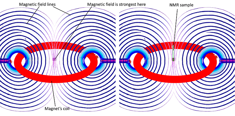
Nuclear magnetic resonance (NMR) is a spectroscopic technique whose energy transitions involve the magnetic spins of atomic nuclei when immersed in a strong magnetic field. This magnetic field is called “static” or “external”, and is literally a very strong magnetic field, thousands of times stronger than the magnetic field of the Earth at the surface. The NMR sample goes right at the core of this strong field:

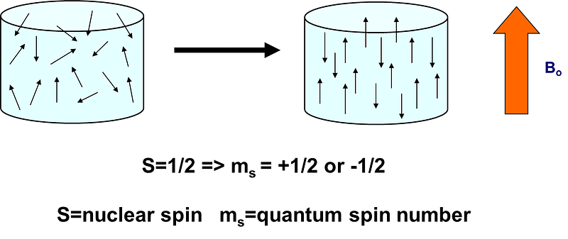
In a classical analogy of a phenomenon that is of intrinsically quantum nature, we can say that NMR-active nuclei behave as tiny magnets that can adopt multiple stable states when immersed in a magnetic field. Each of these states has a slightly different energy, which gives rise to spectroscopy in the form of exciting transitions between these states for each NMR-active nucleus.

Whether the magnetic spin of a nucleus will split into different energy levels or not depends on the magnetic spin number. If it is 0, as in ¹²C, there won’t be any splitting, hence you can’t do any NMR. If it’s 1/2 as in ¹³C, ¹H, ¹⁵N, or ³¹P, then you get two energy levels and you can do NMR. Actually, NMR on these nuclei accounts for the most developed branch of NMR, with the most widely used, standardized applications to chemistry and biology. For those nuclei which can adopt two magnetic states when immersed in a magnetic field, these two states engage “with” or “against” the external magnetic field:

In a sentence, NMR spectroscopy is about promoting transitions between these two states. The “special thing” is that there are so many ways to promote these transitions, to couple them, and to manipulate them as they relax, that then the technique and its theory become very complex (indeed it is “hardcore-complex”, because it’s all rooted in quantum spin physics). But because of the same reasons, the technique is very rich in terms of the information we can derive about molecular systems. And fortunately, you don’t really need to understand all the hardcore physics in detail to make actual use of the technique!

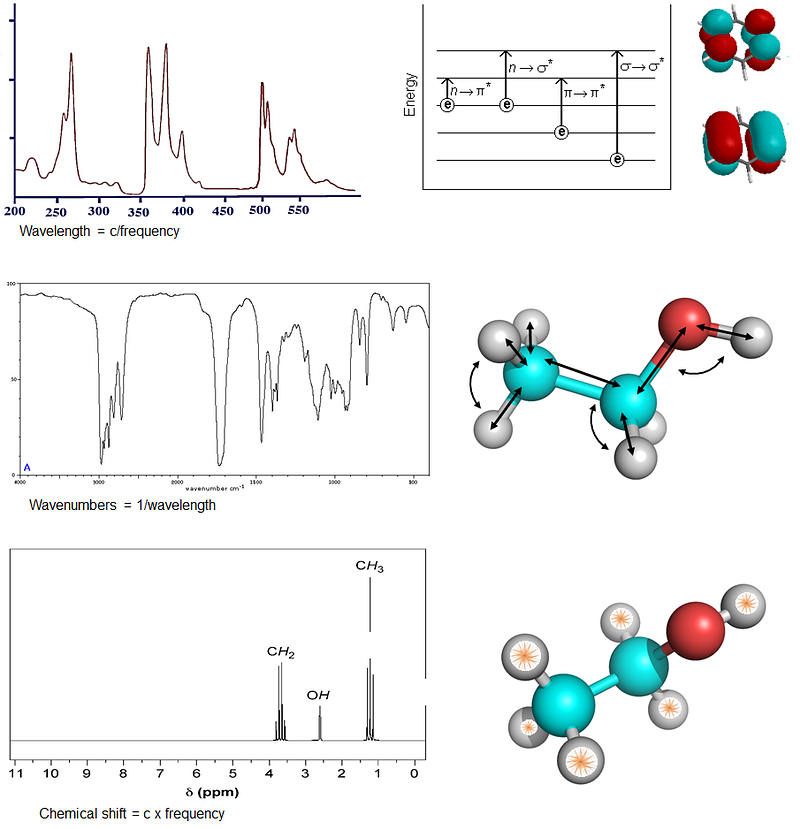
An important point regarding the chemical and structural information that can be derived about a molecule or system by NMR, is that since the NMR phenomenon arises directly from individual transitions in atomic nuclei, the information obtained can achieve atomic resolution. This is in contrast to other spectroscopies which arise from phenomena involving multiple atoms, hence they intrinsically can’t go higher in resolution. For example, absorption spectroscopy reports on the electronic transitions involving whole molecular orbitals hence is informative about the structure of functional groups encompassing many atoms whose electrons make up the involved orbitals. Likewise, infrared spectroscopy reports about the motions of a bunch of atoms connected through bonds. The information coming from NMR is of higher resolution because the core signal comes from individual nuclei (then, couplings of multiple nuclei or convolution of data over multiple can also give lower-resolution information, as we will see in some examples).

Observing NMR signals

To observe NMR signals, scientists need to make sure their samples contain “NMR-active” nuclei -those with magnetic spin > 0 i.e. either 1/2 as in the examples we saw above or higher. The latter pertains to a much less developed, less standardized, and more complex branch of the field; and anyway, applications to biology are largely dominated by studies on spin 1/2 nuclei, on which I focus here.

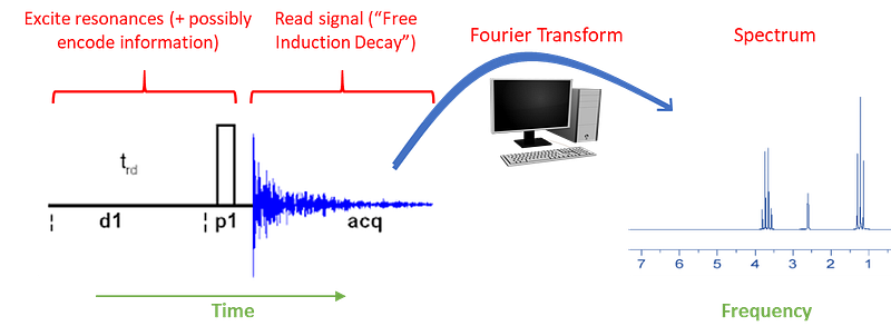
NMR-active nuclei feature specific configurations of protons and neutrons. The right configuration makes them magnetic such that they adopt two or more energy states in the presence of a strong magnetic field. As shown above, in order to do NMR on a sample it must be placed at the core of a very strong magnetic field (reaching 10–20 Tesla, which is thousands of times stronger than the Earth’s magnetic field at the surface). The sample is then irradiated with a series of carefully designed electromagnetic pulses. This set of pulses not just excite the transitions, but they also direct how magnetization “flows” through the different NMR-active nuclei, allowing the detection of links, called “correlations”, between the signals generated by the different nuclei. We’ll touch on this later.

After irradiation, the main NMR “signal” is acquired from the relaxation profile of the excited resonances as they go back to equilibrium, over time. (typically a fraction of a second to some seconds). The resulting time-dependent signal (called FID and which is in the time domain) is processed with a Fourier transform to produce a spectrum of intensities along a frequency axis.

If in solution as in the most common kinds of applications, the NMR spectrum consists of spike-like signals (meaning sharp as opposed to the broad transitions seen in other spectroscopies) that arise from specific excitations at each nucleus, called resonances. Each resonance locates at a quite precise frequency along the x-axis, usually measured in parts per million of deviation relative to a central frequency (hence the units of p.p.m. to measure signal positions by “chemical shift” relative to the reference). The y-axis measures the intensity of each excited resonance, usually dependent not only on concentration but also on a number of factors that are exploited in NMR spectroscopy to probe different aspects about the structure, dynamics and interactions of the target molecule.

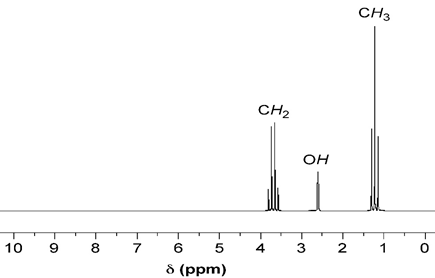
Here is, for example, a 1H NMR spectrum of ethanol, in which you clearly see one main peak for each kind of H atom, with chemical shifts of around 1.1, 2.6, and 3.7 ppm. Notice that each peak is split in different ways; the splitting patterns depend on the covalent connectivities of each H to the nearby Hs, and other factors:

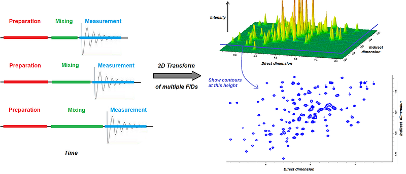
Note that in practice, most of the NMR spectroscopy experiments you will see out there actually happen in “multidimensional mode”, where the signals along two or more frequency axis converge into so-called crosspeaks in 2, 3, or more dimensions. To create these artificial dimensions, the NMR experiments contain variable delays inside the some “mixing periods” during which spins exchange magnetization. By increasing this delay slowly and recording multiple 1D FIDs, one can then compute Fourier transforms along two time dimensions: along the “real” time, to create the normal (called “direct”) frequency dimension, and the time increased inside the mixing periods, to create the “indirect” dimension. By nesting variable delays inside the mixing period, we can augment the number of dimensions further -we’ll see this later with some more detail.

To look at multidimensional spectra, we choose a cutoff for the intensity and then draw contours in say 2 or 3 dimensions. This figure exemplifies how a 2D spectrum is obtained and visualized:

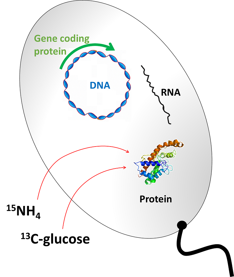
Practically, for organic chemistry and biology, NMR-active nuclei of use in traditional NMR spectroscopy are the abundant ¹H and ³¹P nuclei and the low-abundance ¹³C and ¹⁵N, and in some cases nuclei such as ¹⁹F. When needed, isotopes can be enriched by preparing samples in special ways; for example, proteins for NMR are often produced in a special form that we called “labeled with” or “enriched in” ¹³C and/or ¹⁵N. For this, cells containing a plasmid for regular protein expression are grown in a medium that has sources of ¹³C and/or ¹⁵N as required. The cells then grow and produce the protein enriched in the supplied isotopes; then, a standard purification protocol follows. To produce “labeled proteins” in E. coli, you need to grow the cells in a medium like this one, and induce protein expression in the normal way (just note that reaching cell density good enough for induction of protein expression will take a bit longer than in rich medium, and then expression times are usually longer):

With samples labeled appropriately, and sometimes using the natural abundances of the isotopes, we can acquire and analyze ¹H spectra or say ³¹P or ¹³C spectra in 1D, or combinations of them in 2D such as the ¹H,¹³C HSQC or the ¹H,¹⁵N HSQC, very common in structural studies of proteins. Going to even higher dimensions we can for example have ¹H-¹H correlations resolved in ¹⁵N, as in the ¹⁵N-NOESY or ¹⁵N-TOCSY spectra used to study proteins, or you can also have combinations of multiple nuclei, as in for example the HNCA or HN(CA)CO spectra.

The list of possible spectra is huge, even when single nuclei and single dimensions are involved. Indeed there’s a whole subfield of NMR which is about developing ways to measure such new spectra, that allow the detection and quantification of different properties of a molecular system. We’ll see a few different kinds of spectra throughout the different chapters, so stay tuned.

To move forward, here’s chapter 2

www.lucianoabriata.com I write and photoshoot about everything that lies in my broad sphere of interests: nature, science, technology, programming, etc.

Tip me here or become a Medium member to access all its stories (I get a small revenue without cost to you). Subscribe to get my new stories by email. Consult about small jobs on my services page here. You can contact me here.