MNIST Handwritten Digits Classification using a Convolutional Neural Network (CNN)

The goal of this post is to implement a CNN to classify MNIST handwritten digit images using PyTorch.

This post is a part of a 2 part series on introduction to convolution neural network (CNN).

Part 1 — Basic concepts revolving around CNNs

Part 2 — Pytorch Implementation of a CNN to classify MNIST handwritten digits

This post does not explain working of concepts like convolution layers, max pooling layers, fully connected layers, dropout layers, etc in detail. Read the Part 1 if you are not familiar with them.

You can find the code here — https://github.com/iamkrut/MNIST_handwriting_classification

The MNIST database of handwritten digits, available from this page, has a training set of 60,000 examples, and a test set of 10,000 examples. It is a subset of a larger set available from NIST. The digits have been size-normalized and centered in a fixed-size image.

It is a good database for people who want to learn about various pattern recognition methods for real-world data while spending minimal efforts on pre-processing and formatting.

Fetching the MNIST dataset and preparing train, validation and test data loaders

We can download the dataset from the NIST website but it is more convenient to use the dataset API under torchvision that PyTorch provides, which directly fetches the MNIST data.

We fetch both training and test set made available by NIST. For fetching the training set we set the train argument to True whereas to fetch the test set we set it to False. The dataset API also allows us to address any transformations we want to apply to the data. We set transform=transforms.Compose([transforms.ToTensor()])) to convert the image data to tensors.

mnist_trainset = datasets.MNIST(root='./data', train=True, download=True, 
transform=transforms.Compose([transforms.ToTensor()]))

mnist_testset = datasets.MNIST(root='./data', train=False, download=True, transform=transforms.Compose([transforms.ToTensor()]))

Size of mnist_trainset is 60000 and mnist_testset is 10000

Then we split the test dataset into two sets one for validation and other for testing. We do a 90%–10% i.e. 9000 for validation and 1000 for testing. We use the torch.utils.data.random_split() function to do so.

mnist_valset, mnist_testset = torch.utils.data.random_split(mnist_testset, [int(0.9 *    len(mnist_testset)), int(0.1 * len(mnist_testset))])

After that we prepare data loaders for all three sets. A DataLoader basically combines a dataset and a sampler, and provides an iterable over the given dataset.

It also allows us to pick batch sizes. The batch size is a hyperparameter that defines the number of samples the model looks at before updating the internal model parameters. This concept is called mini-batch gradient descent as the model works on small batches of data to calculate gradients and modifies the model parameters based off them. We choose a batch size of 64 for the train_dataloader , batch size of 32 for val_dataloader and test_dataloader.

train_dataloader = torch.utils.data.DataLoader(mnist_trainset, batch_size=64, shuffle=True)
val_dataloader = torch.utils.data.DataLoader(mnist_valset, batch_size=32, shuffle=False)
test_dataloader = torch.utils.data.DataLoader(mnist_testset, batch_size=32, shuffle=False)

Visualizing the data

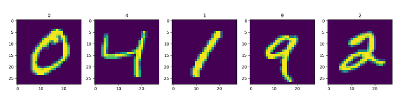
One of the first step while developing a deep learning model is to visualize the data. So let’s plot a few images from the trainset.

This plot shows the digit image along with it’s label on the top. If you print the image data out you can see the values are between 0 and 1. So there is no need to normalize the image data.

Defining the Model

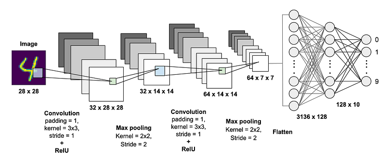
We will define a simple convolutional neural network with 2 convolution layers followed by two fully connected layers.

Below is the model architecture we will be using for our CNN.

We follow up each convolution layer with RelU activation function and a max-pool layer. RelU introduces non-linearity and max-pooling helps with removing noise.

The first convolution layer self.conv_1 takes in a channel of dimension 1 since the images are grayscaled. The kernel size is chosen to be of size 3x3 with stride of 1. The output of this convolution is set to 32 channels which means it will extract 32 feature maps using 32 kernels. We pad the image with a padding size of 1 so that the input and output dimensions are same. The output dimension at this layer will be 32 x 28 x 28.

This is how we define the self.conv_1 layer:

self.conv_1 = torch.nn.Conv2d(in_channels=1, out_channels=32, kernel_size=3, stride=1, padding=1)

The we apply RelU activation to it followed by a max-pooling layer with kernel size of 2 and stride 2. This down-samples the feature maps to dimension of 32 x 14 x 14.

This is how we define the self.relu layer:

self.relu = torch.nn.ReLU()

This is how we define the self.max_pool2d layer:

self.max_pool2d = torch.nn.MaxPool2d(kernel_size=2, stride=2)

The second convolution layer self.conv_2 will have an input channel size of 32. We choose an output channel size to be 64 which means it will extract 64 feature maps. The kernel size for this layer is 3 with stride 1. We again use a padding size of 1 so that the input and output dimension remain the same. The output dimension at this layer will be 64 x 7 x 7.

This is how we define the self.conv_2 layer:

self.conv_2 = torch.nn.Conv2d(in_channels=32, out_channels=64, kernel_size=3, stride=1, padding=1)

We then follow up it with a RelU activation and a max-pooling layer with kernel of size 2 and stride 2. The down-sampled feature map will have dimension 64 x 7 x 7.

We use the same definitionself.relu and self.max_pool2d for this as for self.relu is the same operation and defining it twice makes no sense similarly self.max_pool2d is also the same operation as they use the same kernel size and stride count.

Finally, two fully connected layers self.linear_1 and self.linear_2 are used. We will pass a flattened version of the feature maps to the first fully connected layer. Hence it has to be of dimension 64 x 7 x 7 which is equal to 3136 nodes. This layer will connect to another fully connected layer with 128 nodes. This will be our final layer so the output dimension should match the total classes which is 10. So we have two fully connected layers of size 3136 x 128 followed up by 128 x 10.

This layers self.linear_1 and self.linear_2 are defined as follows:

self.linear_1 = torch.nn.Linear(7 * 7 * 64, 128)
self.linear_2 = torch.nn.Linear(128, 10

Since we want to dropout connections between the two linear layers to reduce overfitting we define self.dropout with a connection dropout probability of 0.5 as follows:

self.dropout = torch.nn.Dropout(p=0.5)

All the above layers and operations are defined under the overridern __init__ method of the class torch.nn.Module

def __init__(self):
    super(Model, self).__init__()
    self.conv_1 = torch.nn.Conv2d(in_channels=1, out_channels=32, kernel_size=3, stride=1, padding=1)
    self.conv_2 = torch.nn.Conv2d(in_channels=32, out_channels=64, kernel_size=3, stride=1, padding=1)
    self.max_pool2d = torch.nn.MaxPool2d(kernel_size=2, stride=2)
    self.linear_1 = torch.nn.Linear(7 * 7 * 64, 128)
    self.linear_2 = torch.nn.Linear(128, 10)
    self.dropout = torch.nn.Dropout(p=0.5)
    self.relu = torch.nn.ReLU()

Next we define how we want the data to flow through these layers by overriding the forward method of the class torch.nn.Module

def forward(self, x):
    x = self.conv_1(x)
    x = self.relu(x)
    x = self.max_pool2d(x)
    x = self.conv_2(x)
    x = self.relu(x)
    x = self.max_pool2d(x)
    x = x.reshape(x.size(0), -1)
    x = self.linear_1(x)
    x = self.relu(x)
    x = self.dropout(x)
    pred = self.linear_2(x)

    return pred

Defining model object, loss function and optimizer

We define an instance of the Model() class and call it model

model = Model()

Loss Criterion: Loss function tells us how good the model is predicting. Since we are dealing with multi class classification we choose cross entropy as our loss function. We use the torch.nn.CrossEntropyLoss which combines a softmax function nn.LogSoftmax() along with nn.NLLLoss() loss function.

criterion = torch.nn.CrossEntropyLoss()

Optimizer: An optimizer ties the loss function and model parameters together by updating the model in response to the output of the loss criterion. We will be using Adam as our optimizer with a learning rate of 0.001.

optimizer = torch.optim.Adam(model.parameters(), lr=0.001)

Training and Valdiation

We will train the model for 100 epochs and pick the model with the lowest validation lost.

Training loop

For each epoch we iterate through batches of train_dataset using an enumerate function over the train_dataloader.

First we set the model to train mode. This allows us to enable the dropout layer and also set the model in training mode.

model.train()

For each batch we pass the batch of image tensors into the model which will return a tensor having predictions for that batch.

pred = model(image)

Having got the predictions we pass them into the cross entropy loss criterion along with their actual labels and calculate the loss.

loss = criterion(pred, label)

We do a backward pass using this loss value and use Adam optimizer to modify the model parameters.

loss.backward()
optimizer.step()

Before each iteration we need to zero out the optimizer gradients.

optimizer.zero_grad()

We get the training loss for the entire epoch by adding all the losses for each batch iteration and averaging it over by the iteration count. Along with that we also keep track of the training loss at each epoch by storing the loss value in a list train_loss

This is what the entire loop looks like:

model.train()
# training
for itr, (image, label) in enumerate(train_dataloader):

    if (torch.cuda.is_available()):
        image = image.cuda()
        label = label.cuda()

    optimizer.zero_grad()

    pred = model(image)

    loss = criterion(pred, label)
    total_train_loss += loss.item()

    loss.backward()
    optimizer.step()

total_train_loss = total_train_loss / (itr + 1)
train_loss.append(total_train_loss)

Validation loop

For each epoch after the training loop we do a validation loop to see how that model performs on the validation set.

First we set the model to eval mode

model.eval()

We then iterate over each batch from the validation dataloader using the enumerate function. We do similar steps as training but we do not backpropagate the loss. After that we compare the model’s prediction with the actual labels and calculate the accuracy of the model. Similar to the training phase, we get the validation loss for the epoch by adding all the losses for each batch iteration and averaging it over by the iteration count. We keep track of validation loss at each epoch by storing the loss value at each epoch in val_loss

This is how the entire loop looks like:

for itr, (image, label) in enumerate(val_dataloader):
    pred = model(image)

    loss = criterion(pred, label)
    total_val_loss += loss.item()

    pred = torch.nn.functional.softmax(pred, dim=1)
    for i, p in enumerate(pred):
        if label[i] == torch.max(p.data, 0)[1]:
            total = total + 1

accuracy = total / len(mnist_valset)

total_val_loss = total_val_loss / (itr + 1)

We plot the training and validation loss for each epoch which are stored under liststrain_loss and val_loss respectively.

fig=plt.figure(figsize=(20, 10))
plt.plot(np.arange(1, no_epochs+1), train_loss, label="Train loss")
plt.plot(np.arange(1, no_epochs+1), val_loss, label="Validation loss")
plt.xlabel('Loss')
plt.ylabel('Epochs')
plt.title("Loss Plots")
plt.legend(loc='upper right')
plt.show()

Below is the train and validation loss plot

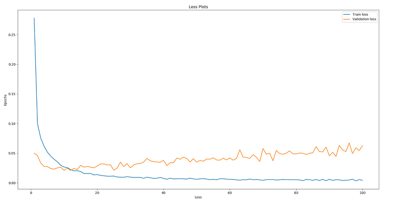
As seen the epoch no. 12 has the lowest validation loss of 0.02092566 and accuracy of 0.99388889 after which the model starts overfitting and the validation loss explodes.

Here is what the training log looks like:

Training dataset size:  60000
Validation dataset size:  9000
Testing dataset size:  1000

Epoch: 1/100, Train Loss: 0.27790789, Val Loss: 0.04998713, Val Accuracy: 0.98311111
Saving the model state dictionary for Epoch: 1 with Validation loss: 0.04998713

Epoch: 2/100, Train Loss: 0.09957011, Val Loss: 0.04592616, Val Accuracy: 0.98533333
Saving the model state dictionary for Epoch: 2 with Validation loss: 0.04592616

Epoch: 3/100, Train Loss: 0.07494711, Val Loss: 0.03318010, Val Accuracy: 0.98900000
Saving the model state dictionary for Epoch: 3 with Validation loss: 0.03318010

Epoch: 4/100, Train Loss: 0.06168462, Val Loss: 0.02777057, Val Accuracy: 0.99033333
Saving the model state dictionary for Epoch: 4 with Validation loss: 0.02777057

Epoch: 5/100, Train Loss: 0.05156403, Val Loss: 0.02722912, Val Accuracy: 0.99100000
Saving the model state dictionary for Epoch: 5 with Validation loss: 0.02722912

Epoch: 6/100, Train Loss: 0.04502778, Val Loss: 0.02404975, Val Accuracy: 0.99233333
Saving the model state dictionary for Epoch: 6 with Validation loss: 0.02404975

Epoch: 7/100, Train Loss: 0.03968575, Val Loss: 0.02311387, Val Accuracy: 0.99211111
Saving the model state dictionary for Epoch: 7 with Validation loss: 0.02311387

Epoch: 8/100, Train Loss: 0.03550077, Val Loss: 0.02516144, Val Accuracy: 0.99188889

Epoch: 9/100, Train Loss: 0.02957717, Val Loss: 0.02641086, Val Accuracy: 0.99144444

Epoch: 10/100, Train Loss: 0.02666702, Val Loss: 0.02112512, Val Accuracy: 0.99344444
Saving the model state dictionary for Epoch: 10 with Validation loss: 0.02112512

Epoch: 11/100, Train Loss: 0.02564372, Val Loss: 0.02457329, Val Accuracy: 0.99266667

Epoch: 12/100, Train Loss: 0.02233217, Val Loss: 0.02092566, Val Accuracy: 0.99388889
Saving the model state dictionary for Epoch: 12 with Validation loss: 0.02092566

Epoch: 13/100, Train Loss: 0.02011606, Val Loss: 0.02414113, Val Accuracy: 0.99322222

Epoch: 14/100, Train Loss: 0.02053968, Val Loss: 0.02243329, Val Accuracy: 0.99388889

.
.
.

Epoch: 99/100, Train Loss: 0.00538922, Val Loss: 0.05434694, Val Accuracy: 0.99366667

Epoch: 100/100, Train Loss: 0.00425748, Val Loss: 0.06263806, Val Accuracy: 0.99288889

Testing and Visualizing results

We fetch the saved model state dictionary for the model having the lowest validation loss and load it up into our model. Next we set the model to eval mode.

model.load_state_dict(torch.load("model.dth"))
model.eval()

We enumerate through our test dataloader and calculate the models accuracy the same way we did with the validation loop. We also store the results in a “results” list. With this model I got 0.99300000 accuracy on the test set.

results = list()
total = 0
for itr, (image, label) in enumerate(test_dataloader):
    pred = model(image)
    pred = torch.nn.functional.softmax(pred, dim=1)

    for i, p in enumerate(pred):
        if label[i] == torch.max(p.data, 0)[1]:
            total = total + 1
            results.append((image, torch.max(p.data, 0)[1]))

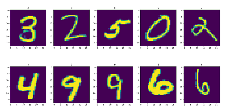
We then plot the results.

# visualize results
fig=plt.figure(figsize=(20, 10))
for i in range(1, 11):
    img = transforms.ToPILImage(mode='L')(results[i]             [0].squeeze(0).detach().cpu())
    fig.add_subplot(2, 5, i)
    plt.title(results[i][1].item())
    plt.imshow(img)
plt.show()

The predicted label is shown above each image. As we can see from the results our model is predicting well.

Disclaimer

While this post covers the implementation of a CNN model in pytorch to classify MNIST handwritten digits, it is by no means the best implementation to do so. The performance can be further improved using data augmentation, tuning dropout layers, regularization, batch normalization, hyper-parameter tuning. etc. It was aimed towards beginners who are trying to get into computer vision and want to start off from somewhere.