Convolutional Neural Networks — A Beginner’s Guide

The goal of this post is to serve as a introduction to basic concepts involved in a convolution neural network. This post is focused towards the final goal of implementing a MNIST handwritten digit classifier so everything is explained keeping that in mind — convolution layers, max pooling layers, RelU activation function, fully connected layers, dropout layers, cross entropy loss function, etc.

This post is a part of a 2 part series on introduction to convolution neural network (CNN).

Part 1 — Basic concepts revolving around CNNs

Part 2 — Pytorch Implementation of a CNN to classify MNIST handwritten digits

1. Convolution Layer

Before digging into what a convolution layer is, let’s understand why use them in the first place.

Why use a Convolution Layer?

Before the concept of convolution was presented by Yann LeCun in 1998 for digit classification, people used other methods like support vector machine, knn, logistic regression, etc to classify images. In those algorithms, pixel values were considered as features i.e. for a 28x28 image there would be 784 features.

There are a lot of algorithms that people used for image classification before convolution became popular. People used to create features from images and then feed those features into some classification algorithm like SVM. Some algorithms also used the pixel level values of images as a feature vector. To give an example, you could train a SVM with 784 features where each feature is the pixel value for a 28x28 image. This way we lose a lot of spatial interaction between pixels. We could still handpick features out of the image similar to what a convolution layer automatically does, but it would be much time intensive. Convolution layer uses information from adjacent pixels to down-sample the image into features by convolution and then use prediction layers to predict the target values.

How does a Convolution layer work?

We use multiple convolution filters or kernels that run over the image and compute a dot product. Each filter extracts different features from the image.

Lets consider a filter of size 3x3 and an image of size 5x5. We perform an element wise multiplication between the image pixel values that match the size of the kernel and the the kernel itself and sum them up. This provides us a single value for the feature cell.

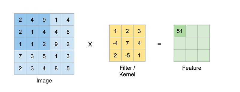
2*1 + 4*2 + 9*3 + 2*(-4) + 1*7 + 4*4 + 1*2 + 1*(-5) + 2*1 = 51

Filter continues to run further on the image and produce new values as shown below.

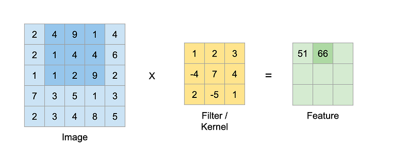
4*1 + 9*2 + 1*3 + 1*(-4) + 4*7 + 4*4 + 1*2 + 2*(-5) + 9*1 = 66

and so on …

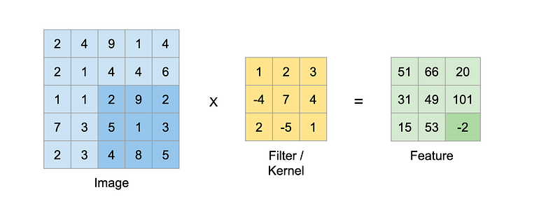
2*1 + 9*2 + 2*3 + 5*(-4) + 1*7 + 3*4 + 4*2 + 8*(-5) + 5*1 = -2

In the above example we are sliding the kernel by 1 pixel. This is called stride. We can have the kernel move by different stride values to extract different kinds of features.

Also the amount of stride we choose affects the size of the feature extracted. The equation to calculate the size of feature for a particular kernel size is as follows:

Feature size = ((Image size − Kernel size) / Stride) + 1

We can put the values for the above example and verify it.

Feature size = ((5 − 3) / 1) + 1 = 3

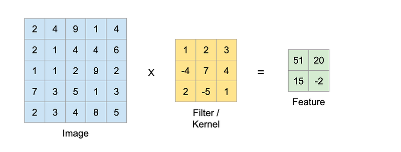
So with a stride of 2 the kernel of size 3x3 on a image of size 5x5 would only be able to extract a feature of size 2.

What if you want the feature to be of the same size as the input image? You can achieve this by padding the image. Padding is a technique to simply add zeros around the margin of the image to increase it’s dimension. Padding allows us to emphasize the border pixels and in order lose less information.

Here is an example with an input image of size 5x5 which is padded to 7x7 i.e. padding size of 1 and convoluted by a kernel of size 3x3 with stride of 1 resulting in a feature of size 5x5.

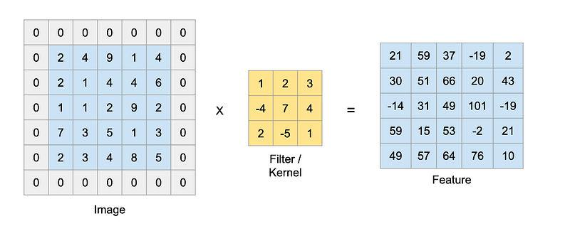
The equation to calculate the size of feature for a particular kernel size when considering a padded image is as follows:

Feature size = ((Image size + 2 * Padding size − Kernel size) / Stride)+1

We can put in the values for the above example and verify it.

Feature size = ((5 + 2 * 1 − 3) / 1) + 1= 5

For an image with 3 channels i.e. rgb we perform the same operation on all the 3 channels.

A neural network learns those kernel values through back propogation to extract different features of the image. Typically in a convolutional neural network we would have more than 1 kernel at each layer. We can further use those feature maps to perform different tasks like classification, segmentation, object detection etc.

Here are some nice visualizations for a convolution layer -

2. Max Pooling Layer

Max pooling layer helps reduce the spatial size of the convolved features and also helps reduce over-fitting by providing an abstracted representation of them. It is a sample-based discretization process.

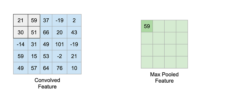
It is similar to the convolution layer but instead of taking a dot product between the input and the kernel we take the max of the region from the input overlapped by the kernel.

Below is an example which shows a maxpool layer’s operation with a kernel having size of 2 and stride of 1.

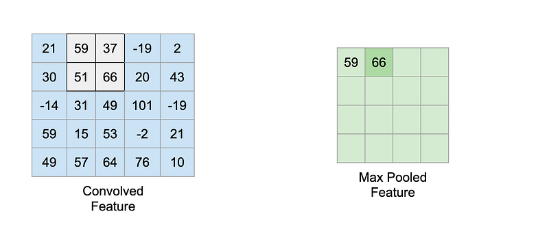
and so on …

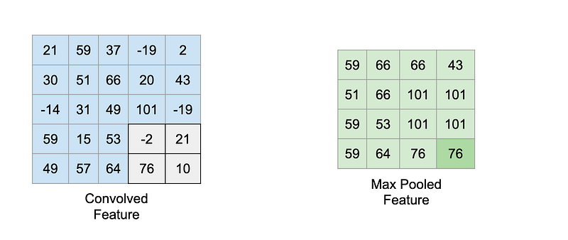
There is one more kind of pooling called average pooling where you take the average value instead of the max value. Max pooling helps reduce noise by discarding noisy activations and hence is better than average pooling.

3. RelU (Rectified Linear Unit) Activation Function

Activation functions introduce non-linearity to the model which allows it to learn complex functional mappings between the inputs and response variables. There are quite a few different activation functions like sigmoid, tanh, RelU, Leaky RelU, etc.

RelU function is a piecewise linear function that outputs the input directly if is positive i.e. > 0, otherwise, it will output zero.

ReLU(x)=max(0,x)

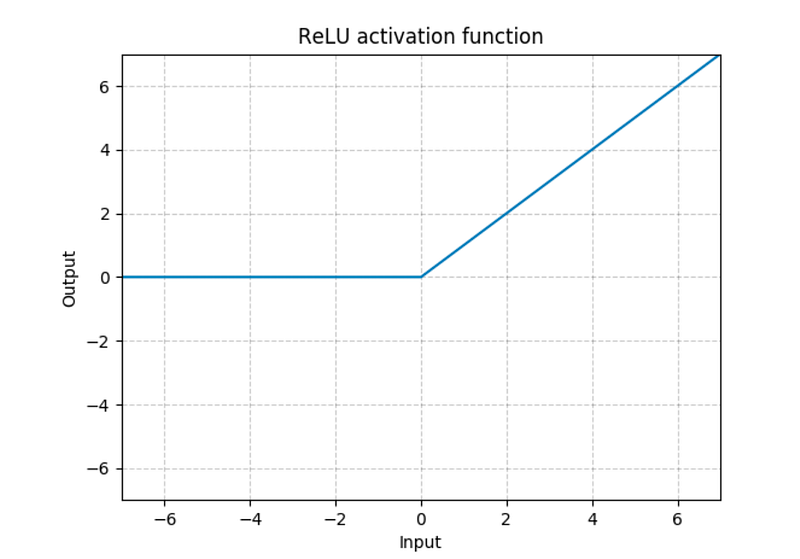
There are many other activation functions but RelU is the most used activation function for many kinds of neural networks as because of it’s linear behavior it is easier to train and it often achieves better performance.

RelU activation after or before max pooling layer

Well, MaxPool(Relu(x)) = Relu(MaxPool(x))

So they satisfy the communicative property and can be used either way. In practice RelU activation function is applied right after a convolution layer and then that output is max pooled.

4. Fully Connected layers

In a fully connected layer the input layer nodes are connected to every node in the second layer. We use one or more fully connected layers at the end of a CNN. Adding a fully-connected layer helps learn non-linear combinations of the high-level features outputted by the convolutional layers.

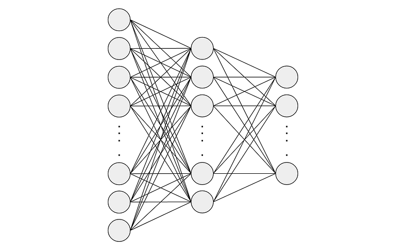
Usually, activation function and dropout layer are used between two consecutive fully connected layers to introduce non-linearity and reduce over-fitting respectively.

At the last fully connected layer we choose the output size based on our application. For classifying the MNIST handwritten digits the last layer will be of size 10 i.e. one node for each digit and we will take a softmax of the output which gives us a 10 dimensional vector containing probabilities (a number ranging from 0–1) for each of the digits.

5. Dropout layer

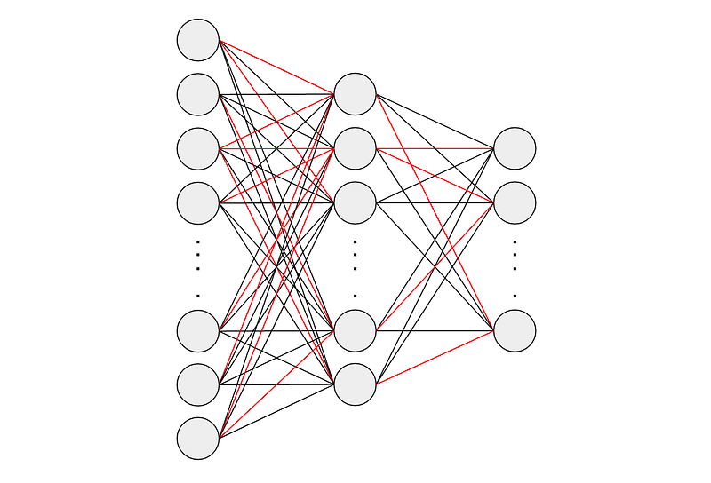
Dropout is a regularization technique used to reduce over-fitting on neural networks. Usually, deep learning models use dropout on the fully connected layers, but is also possible to use dropout after the max-pooling layers, creating image noise augmentation.

Dropout randomly zeroes some of the connections of the input tensor with probability p using samples from a Bernoulli distribution.

6. Loss function — Cross Entropy

A loss function is a method of evaluating how well the model models the dataset. The loss function will output a higher number if the predictions are off the actual target values whereas otherwise it will output a lower number.

Since our problem is of type multi-class classification we will be using cross entropy as our loss function. It basically outputs a higher value if the predicted class label probability is low for the actual target class label.

Disclaimer

While this post covers most of the concepts revolving around a CNN model used to classify images, it is by no means a comprehensive guide. It is focused towards beginners and the final goal is to implement a CNN MNIST handwritten data classifier.

In the next part Part 2 — Pytorch Implementation of a CNN to classify MNIST handwritten digits we will putting all these concepts to use by implementing a Convolutional Neural Network (CNN) network to classify MNIST Handwritten Digits.