
Maximize Your Stock Market Earnings With Machine Learning
The A-Z guide on how to maximize the efficiency of a stock-investing portfolio using ML.

The first part of the series can be found here.
The objective of this two-part series is to build a Machine Learning model that will evaluate the recommendations provided by Yahoo Finance Analysts on the basis of public sentiment for the company on Twitter and Financial News. After performing the analysis, the model will inform the user of whether he/she should buy the stock, building this way, an efficient investing portfolio.
In the first part, we set-up the majority of system functions and made a fully operational model. In particular, the steps followed were the following:
- Fetch the stock names recommended by Yahoo Finance.
- Fetch all possible News Articles related to those companies.
- Fetch all possible tweets related to those companies.
- Combine all tweets and articles into two separate strings.
- Perform sentiment analysis on the Tweets and News Articles.
- According to that score, dictate whether the Analysts’ recommendations should be followed.
- Send the final recommendations to the user via Facebook messenger.
If one wants to truly make money using Machine Learning, there are some additional things that much be done. In particular, we are interested in maximizing profit by partitioning our holdings in the best way possible.
If you want to be able to order articles of your own, access exclusive content, and receive free products created by me to empower your Business (including much more), do not hesitate to visit my Patreon.
Project Blueprint

So what is the objective of this article?
The objective is clear, I will be using the final stocks recommendations from Part 1, and I will be building a model that is going to estimate the best way to partition our portfolio, in order to maximize the possible returns and at the same time minimize risk.
In order to select the best possible asset distribution, we will be relying on the “Sharpe Ratio” (see keywords). The ratio describes how much excess return you receive for the extra volatility you endure for holding a riskier asset.
It is generally accepted that a Sharp Ratio of “1” is considered optimal. “2” is really desirable, and “3” is extremely optimal.
According to this premise, we will be using the Machine Learning generated predictions and will maximize our potential profits.
Continue reading to see how you can maximize your earnings using this simple method!
Keywords
Having a precise plan in mind, we can now proceed by creating the model. Before doing so, I will be defining some simple financial terms that will be used throughout the analysis.
Portfolio Variance
According to Investopedia:
Portfolio variance is a measurement of risk, of how the aggregate actual returns of a set of securities making up a portfolio fluctuate over time. This portfolio variance statistic is calculated using the standard deviations of each security in the portfolio as well as the correlations of each security pair in the portfolio.
In simpler terms, it is used as a measurement of risk.
Sharpe Ratio
The Sharp Ratio is essentially a tool with which you can find the best possible proportion to allocate to each stock in a portfolio.
Covariance Matrix
In essence, the covariance matrix is used as a means of determining how much two random variables move together or vary. It is commonly used when comparing data samples from different sources. In this case scenario, it is the directional relationship between the price of two assets.
For more information, check this website.
If you like this article and are interested in receiving exclusive monthly content for free, subscribe to my exclusive mailing list at the end of this article (can be also accessed directly from here).
Performing The Analysis
*I will start from where I finished in the first part. Nevertheless, you could add whatever stock you wanted manually here, and just follow along.
The first step is to import all of the required libraries.
For the shake of convenience, I will be creating a list called “assets” which will contain all of the values in the “tickers” array (the tickers of the final stocks that resulted from Part 1). I will be also setting the weights as 0.066 each.
I will be setting the start date for the historical stocks-prices as the first of January, 2016. To import the prices, Yahoo Finance is going to be used.
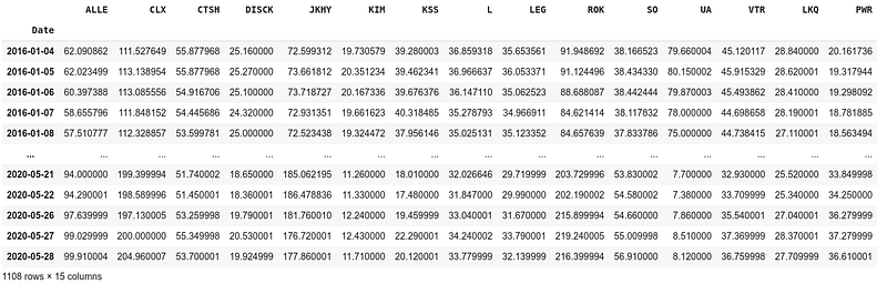
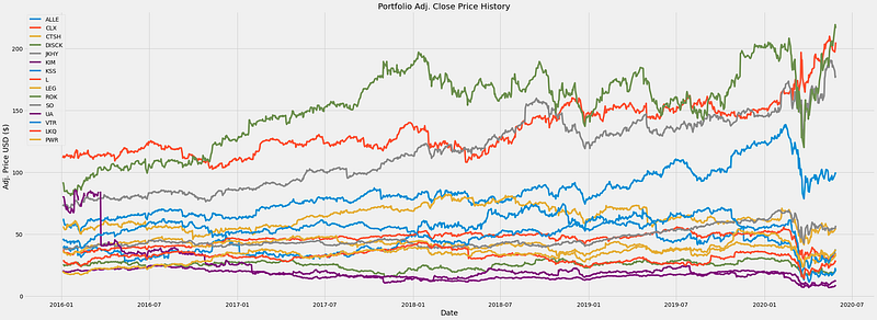
Perfect! Everything seems to be imported correctly. It is now time to plot the different prices on a graph.
Performing Financial Calculations
Our fictional portfolio is ready. It is now time to perform some sample calculations.
To start with, I will be calculating the daily simple returns by using the following formula:
(new_price/old_price) / old_priceThis can be done with the following line of code:
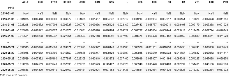
Simple, yet effective! Lets now calculate the co-variance matrix.
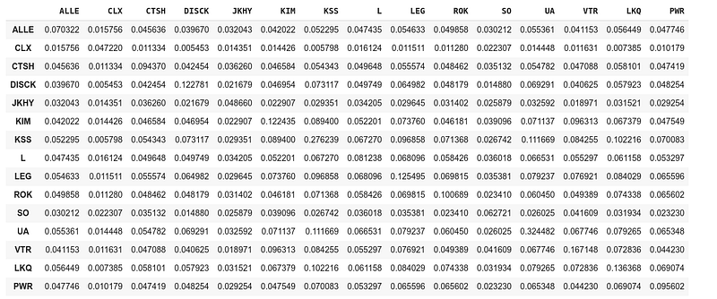
The portfolio variance is another useful measurement. The formula to calculate it is quite simple and can be incorporated in python as follows:
Finally, it is crucial that we calculate the volatility (square root of the variance), and the portfolio annual simple return.
At the stage, three measurements are of importance for this model:
- Expected Annual Return
- Annual Volatility (Risk)
- Annual Variance
For the current model, these figures are:
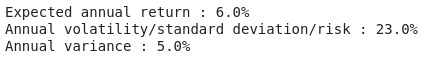
It appears that the annual return is at 6% and the risk is 23%. According to most investors’ standards, this would certainly not be desirable. This is where portfolio optimization comes in.
Portfolio Optimization
Thankfully, there is a library called “pypfopt” that can automate the entire process on our behalf.
As a reminder, to use pypfopt, the following should be imported:
from pypfopt.efficient_frontier import EfficientFrontier
from pypfopt import risk_models
from pypfopt import expected_returns
from pypfopt.discrete_allocation import DiscreteAllocation, get_latest_prices
To calculate the expected returns and annualized sample variance matrix of daily returns, only two lines of code are needed.
It is now finally time to optimize the portfolio for maximum Sharpe ration.

Voila! The expected annual return has now increased to 21.1% and the risk has decreased to 17.9%.
We will now be setting our budget of $15,000 and will be asking the model to tell us how to allocate it effectively (according to current prices).

The model has now completed. It appears, that the best way to partition the portfolio is by owning:
22 CLX Stocks
43 JKHY Stocks
13 ROK Stocks
1 KSS Stocks
1 UA Stocks
Not only do we have an optimized portfolio to maximize profits, but we also have some money left to spend for ourselves!
Do you want to learn more?
If you want to advance your knowledge and are interested in making money using Machine Learning I highly encourage you to follow me and read the articles listed below:


