Fine-Tuning ViT on Custom Datasets for Image Classification | By Gaurav Gupta

Problem Statement

Greetings, fellow AI enthusiasts! 👋

As a dedicated learner in the realms of Machine Learning and Artificial Intelligence for the past two years, I have immersed myself in the complexities of training Transformer Models. However, like many practitioners in the field, I’ve encountered a common challenge in the corporate landscape: training Transformer Models on custom datasets. These datasets, collected in real-time rather than sourced from established platforms, present unique obstacles.

In this article, I aim to tackle this challenge head-on by exploring how we can effectively train Vision Transformer models on custom datasets. Let’s dive in!

Procedure

Ready to master Vision Transformer (ViT) for custom image classification? Let’s break it down into six simple steps:

1. Data Collection: Prepare your dataset for action.
2. Dataset Loading: Utilize HuggingFace 🤗 for seamless dataset loading.
3. Loading Pre-trained ViT: Introduce the pre-trained ViT model to your project.
4. Model Training: Dive into training and fine-tuning your model.
5. Model Testing: Evaluate your model’s performance and watch it shine.
6. Model Prediction: Use the power of code to make predictions with your trained model.

STEP 1: DATA COLLECTION

Alert: If your dataset is already available on HuggingFace 🤗, skip ahead to Step 2! Otherwise, follow these simple instructions to gather and organize your data for loading into the model:

1. Collect or Download Images: Gather all your training and testing images from your preferred source, such as Kaggle.
2. Create a Root Directory: Set up a folder named custom_dataset to serve as the main directory for your dataset.
3. Create Sub-folders for Labels: Inside the custom_dataset folder, create sub-folders named after the labels or classes you've defined.
4. Organize Your Images: Place your images into their respective sub-folders. For example, if you’re training a model to classify checkboxes into categories like correct, wrong, and empty, create three sub-folders within the custom_dataset directory—correct, wrong, and empty. Each folder should contain images representing its corresponding class.

By following these steps, you’ll have a well-organized dataset ready for the next phase.

STEP 2: DATASET LOADING

Before diving into loading your dataset with HuggingFace 🤗, let’s set up the environment. Whether you’re working in Jupyter or Google Colab, run the following script to ensure you have all the necessary packages installed:

!pip install datasets 
!pip install -U accelerate
!pip install -U transformers
!pip install scikit-learn pillow torchvision opencv-python

Case 1: Loading a Dataset from HuggingFace

If your dataset is available on HuggingFace 🤗, loading it is a breeze. Use the load_dataset function as shown below:

from datasets import load_dataset

# replace 'cifar10' with the name of your dataset
dataset = load_dataset("cifar10")

Case 2: Loading Your Custom Dataset

For those of you working with your data, follow these steps to prepare and load your custom dataset:

• Import Necessary Libraries:

from sklearn.model_selection import train_test_split
from datasets import load_dataset, DatasetDict, load_metric

• Specify the Root Directory:

root_dir = 'path/to/custom_dataset'  # enter the path where your 'custom_dataset' folder is stored

• Load the Dataset:

ds = load_dataset("imagefolder", data_dir=root_dir)

• Split the Dataset into Training and Testing Sets:

ds = ds['train'].train_test_split(test_size=0.3, stratify_by_column="label")  # 70% train, 30% test
ds_test = ds['test'].train_test_split(test_size=0.5, stratify_by_column="label")  # 30% test --> 15% valid, 15% test
ds = DatasetDict({
    'train': ds['train'],
    'test': ds_test['test'],
    'valid': ds_test['train']
})

del ds_test

• Verify the Dataset:

ds

# EXPECTED OUTPUT

Resolving data files: 100%
  2088/2088 [00:00<00:00, 16116.71it/s]
Downloading data: 100%
  2088/2088 [00:00<00:00, 16777.02files/s]
Generating train split: 
  2088/0 [00:00<00:00, 3318.34 examples/s]
DatasetDict({
    train: Dataset({
        features: ['image', 'label'],
        num_rows: 1461
    })
    test: Dataset({
        features: ['image', 'label'],
        num_rows: 314
    })
    valid: Dataset({
        features: ['image', 'label'],
        num_rows: 313
    })
})

STEP 3: Loading a Pre-trained ViT

In this step, we’ll harness the power of HuggingFace 🤗’s transformer library to load a pre-trained Vision Transformer (ViT) model. Let’s streamline the process with a couple of handy functions.

• Extracting Labels from Our Dataset

First, we need to extract the labels from our dataset:

labels = ds['train'].features['label']
labels

# SAMPLE OUTPUT

ClassLabel(names=['correct', 'empty', 'wrong'], id=None)

• Defining the Transform Function

Next, let’s define a transform function to prepare our images for model input. Remember, tailoring the transformation to match the pre-trained model’s requirements is crucial for optimal performance.

from PIL import Image
import torchvision.transforms as transforms

def transform(example_batch):
    # Define the desired image size
    desired_size = (224, 224)

    # Resize the images to the desired size
    resized_images = [transforms.Resize(desired_size)(x.convert("RGB")) for x in example_batch['image']]

    # Convert resized images to pixel values
    inputs = processor(resized_images, return_tensors='pt')

    # Don't forget to include the labels!
    inputs['label'] = example_batch['label']

    return inputs

prepared_ds = ds.with_transform(transform)

• Defining the Collate Function and Metric Function

Let’s define the collate function and the metric function to handle our batches and compute the accuracy of our model:

def collate_fn(batch):
    return {
        'pixel_values': torch.stack([x['pixel_values'] for x in batch]),
        'labels': torch.tensor([x['label'] for x in batch])
    }

metric = load_metric("accuracy")

def compute_metrics(p):
    return metric.compute(predictions=np.argmax(p.predictions, axis=1), references=p.label_ids)

• Loading the Pre-trained ViT Model

Finally, let’s load the pre-trained Vision Transformer model:

from transformers import AutoImageProcessor, ViTForImageClassification

model_name_or_path = 'google/vit-base-patch16-224-in21k'

processor = AutoImageProcessor.from_pretrained(model_name_or_path)
model = ViTForImageClassification.from_pretrained(
    model_name_or_path,
    num_labels=len(labels),
    id2label={str(i): c for i, c in enumerate(labels)},
    label2id={c: str(i) for i, c in enumerate(labels)},
    ignore_mismatched_sizes=True
)

You might encounter some warnings regarding mismatched sizes, but don’t worry — you can safely ignore them. Now, we’re ready to move on to the next step and start training our model!

# OUTPUT

/usr/local/lib/python3.10/dist-packages/huggingface_hub/file_download.py:1132: FutureWarning: `resume_download` is deprecated and will be removed in version 1.0.0. Downloads always resume when possible. If you want to force a new download, use `force_download=True`.
  warnings.warn(
Some weights of ViTForImageClassification were not initialized from the model checkpoint at google/vit-base-patch16-224-in21k and are newly initialized: ['classifier.bias', 'classifier.weight']
You should probably TRAIN this model on a down-stream task to be able to use it for predictions and inference.

STEP 4: Model Training

Now, it’s time to fine-tune our pre-trained Vision Transformer (ViT) model. By defining hyperparameters and initiating the training process, we’ll bring our model closer to perfection.

• Setting Up Hyperparameters

First, replace root_dir with the actual path where you want to save all model configuration files and checkpoints. Then, set up the hyperparameters for training:

from transformers import TrainingArguments

root_dir = "/ViT_custom/"  # Path where all config files and checkpoints will be saved
training_args = TrainingArguments(
  output_dir=root_dir,
  per_device_train_batch_size=16,
  evaluation_strategy="epoch",
  save_strategy="epoch",
  fp16=True,
  num_train_epochs=20,
  logging_steps=500,
  learning_rate=2e-4,
  save_total_limit=1,
  remove_unused_columns=False,
  push_to_hub=False,
  report_to='tensorboard',
  load_best_model_at_end=True,
)

• Defining the Trainer

Next, let’s define the trainer. This will take the hyperparameters, optimizers, and training/validation datasets as input:

from transformers import Trainer

trainer = Trainer(
    model=model,
    args=training_args,
    data_collator=collate_fn,
    compute_metrics=compute_metrics,
    train_dataset=prepared_ds["train"],
    eval_dataset=prepared_ds["valid"],
    tokenizer=processor,
)

• Kicking Off the Training Process

Now, let’s kick off the training process. Define the path to save the best model, then start training:

save_dir = '/path/to/ViT_custom/best_model/'  # Define the path to save the model
train_results = trainer.train()
trainer.save_model(save_dir)  # Save the best model
trainer.log_metrics("train", train_results.metrics)
trainer.save_metrics("train", train_results.metrics)
trainer.save_state()

The above code will automatically save the best model in the best_model folder within the root directory. Get ready to witness your model evolve and improve with each epoch!

STEP 5: Model Testing

The moment of truth has arrived — let’s put our model to the test and see how well it performs on various metrics using our test dataset. Follow these steps to evaluate and visualize the model’s performance:

• Evaluate the Model

First, execute the script below to evaluate your model and log the metrics:

metrics = trainer.evaluate(prepared_ds['test'])
trainer.log_metrics("test", metrics)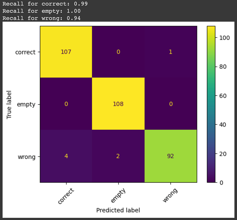
trainer.save_metrics("test", metrics)

• Generate Confusion Matrix and Recall Scores

To delve deeper into the model’s performance, we’ll use the sklearn library to create a confusion matrix and calculate recall scores for each class:

from sklearn.metrics import confusion_matrix, ConfusionMatrixDisplay, recall_score

test_ds = ds['test'].with_transform(transform)
test_outputs = trainer.predict(test_ds)

y_true = test_outputs.label_ids
y_pred = test_outputs.predictions.argmax(1)

labels = test_ds.features["label"].names
cm = confusion_matrix(y_true, y_pred)
disp = ConfusionMatrixDisplay(confusion_matrix=cm, display_labels=labels)
disp.plot(xticks_rotation=45)

recall = recall_score(y_true, y_pred, average=None)

# Print the recall for each class
for label, score in zip(labels, recall):
  print(f"Recall for {label}: {score:.2f}")

• Visualize Performance

Here’s what the confusion matrix and recall scores will look like:

STEP 6: Model Prediction

Now that our model is trained and tested, it’s time to put it to work! We’ll define a function to make predictions on new images using our fine-tuned Vision Transformer (ViT) model.

• Define the Prediction Function

First, create a function to handle the prediction process:

def getPrediction(image):
    model_name_or_path = 'google/vit-base-patch16-224-in21k'
    processor = AutoImageProcessor.from_pretrained(model_name_or_path)
    vit = ViTForImageClassification.from_pretrained(save_dir)
    model = pipeline('image-classification', model=vit, feature_extractor=processor)
    
    result = model(image)
    return result

• Use the Function to Predict

Replace '…/path/to/image.jpg' with the actual path to your image file. Then, run the following code to get the prediction:

import cv2

image = cv2.imread(".../path/to/image.jpg")
print(getPrediction(image))

With this function, you can now effortlessly predict the class of any new image. It’s as simple as that!

Comments and Thanks

Thank you for taking the time to read my very first article on Medium.

I hope you found it helpful and informative. If you have any doubts, questions, or feedback, please feel free to leave a comment below. Your input is highly appreciated and will help me improve. If you liked this article or found it useful, I would love to hear your thoughts. Thanks again for your support!

Until next time, happy coding and may your models shine brightly! 🌟

References

Related Articles