ViT: Vision Transformer
Transformers for image recognition at scale.
Blog by Anuja Bhajibhakre and Shivani Junawane
If you like a video presentation please refer to the youtube video link: https://www.youtube.com/watch?v=tRQ0EaqeJAI&t=1s
Implementation: https://github.com/junawaneshivani/VisionTransformer/blob/main/vit_from_scratch.ipynb
Transformer architectures as introduced in the “ATTENTION IS ALL YOU NEED” paper have had huge impacts in the NLP domain. But, its applications in the Computer Vision domain had been limited. In 2021, a research team at Google introduced the paper “AN IMAGE IS WORTH 16X16 WORDS: TRANSFORMERS FOR IMAGE RECOGNITION AT SCALE (2021)”, which applied the Transformer encoder architecture to the image recognition(classification) task.
Idea of the paper:
The idea of the paper is to create a Vision Transformer using the Transformer encoder architecture, with the fewest possible modifications, and apply it to image classification tasks.
When Vision Transformers(ViT) are trained on sufficiently large amounts of data (>100M), with much fewer computational resources(four times less) than the state-of-the-art CNN (ResNet), and transferred to multiple mid-sized or small image recognition benchmarks, it attains excellent results. The results are further discussed in detail in the last sections of the blog.
Now, that we have an idea of the paper, let us first define our goal.
Goal:
Image Classification
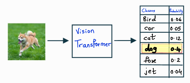
Image classification deals with assigning a class label to the input image. For example, as you can see in the below image, we predict the class as Dog for our input image as it has the highest confidence score after applying softmax.
The Vision Transformer
The below diagram shows the Vi(sion) T(ransformer) architecture.
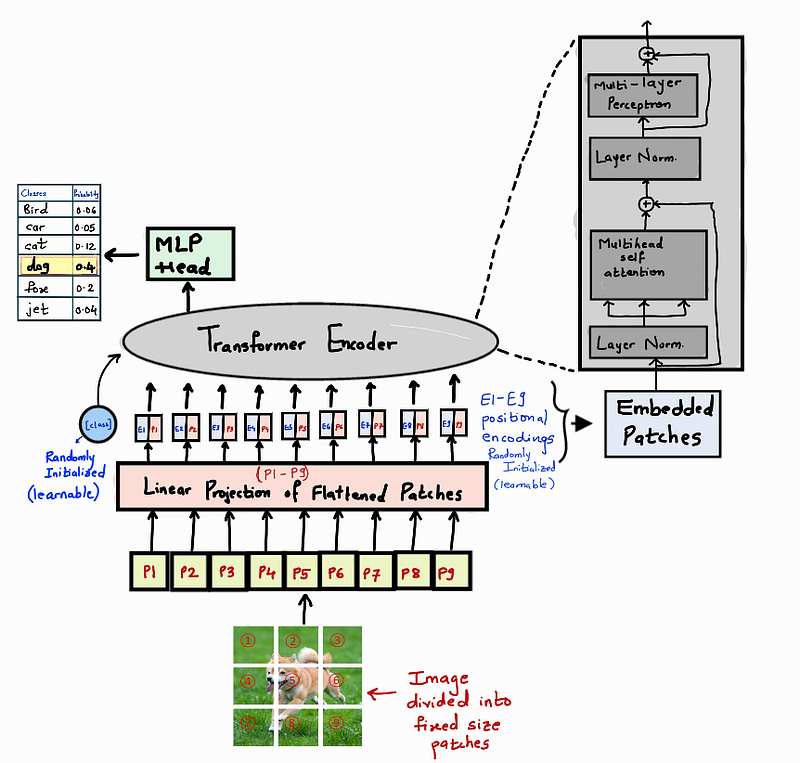
To understand the architecture better, let us divide it into 3 components.
- Embedding
- Transformer Encoder
- MLP Head
Step 1: Embedding
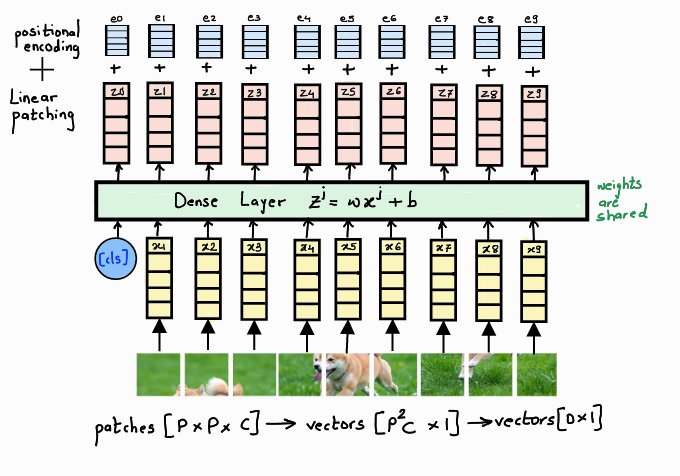
In this step, we divide the input image into fixed-size patches of [P, P] dimension and linearly flatten them out, by concatenating the channels (if present). For example, a patch of size [P, P, C] is converted to [P*P*C, 1]. This linearly flattened patch is further passed through a Feed-Forward layer with a linear activation function to get a linear patch projection of the dimension [D, 1]. D is the hyperparameter called as embedding dimension used throughout the transformer.
The image can be patched using a Convolutional Layer by keeping the stride equal to the patch size. This will convert the input image into patches of the required size, which are then flattened and passed to the next layer.
For classification purposes, taking inspiration from the original BERT paper, we concatenate a learnable class embedding with the other patch projections, whose state at the output serves as class information. This extra class token is added to the set of image tokens which is responsible for aggregating global image information and final classification. It is able to learn this global aggregation while it passes and learns through the attention layers. We also add a 1D positional embedding to the linear patches, to establish a certain order in the input patches.
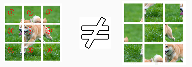
Why is positional encoding necessary?
Transformers are not capable of remembering the order or sequence of the inputs. If the image patches are re-ordered the meaning of the original image is lost. Hence, we add a positional embedding to our linearly embedded image patches to keep track of the sequence.
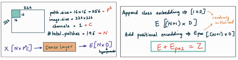
To understand the embedding step a bit better let us see the dimensions.
Suppose, we have an input image of size 224x224x1, we divide it into fixed-size patches of size 16x16. Let us denote the patch size as P and the image channels as C. The total number of patches N that we get is 196.
After linearly flattening all the patches to get a vector X of dimension [N, P²C]., we pass it through a Dense Layer to convert it to a D dimensional vector called embedding E [N, D]. We then append a learnable class embedding [1, D] to convert the E vector to dimension [N+1, D]. The last step is adding positional encoding to get the final vector Z. Both the class and positional embeddings are randomly initialized vectors, learned during the training of the network.
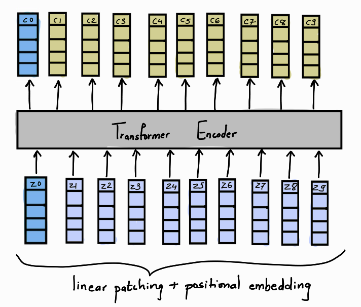
Once we have our vector Z we pass it through a Transfomer encoder layer.
Step 2: Transformer Encoder
The Transformer Encoder architecture is similar to the one mentioned in the “ATTENTION IS ALL YOU NEED” paper. It is composed of multiple stacks of identical blocks. Each block has a Multi-Head Attention layer followed by a Feed-Forward layer. There is a residual connection around each of the two sub-layers, followed by layer normalization. All sub-layers as well as the embedding layers in the model produce an output of embedded dimension D. The Z vector from the previous step is passed through the transformer Encoder architecture to get the context vector C.
The Transformer Encoder architecture consists of multiple encoder blocks, where each block has a Multi-Head Attention unit and a Feed-Forward Network. Each layer is also followed by a normalization layer.
Assuming that we already are aware of the mechanism of a Feed-Forward layer, let us look at the Multi-Head Attention.
Multi-Head Attention:
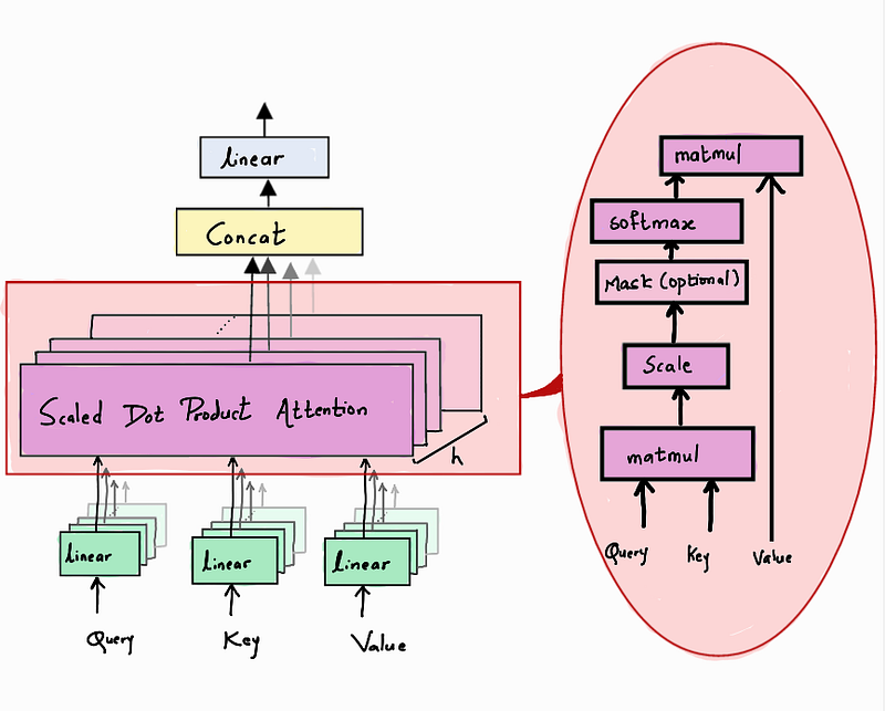
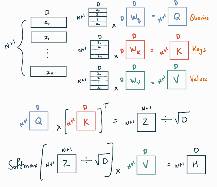
The main component of a Multi-Head Attention unit is the Scaled Dot-Product Attention. At first, the input vector Z is duplicated 3 times and multiplied by weights Wq, Wk, and Wv, to get the Queries, Keys, and Values respectively. The Queries are then multiplied by the Keys, and the result is divided by the square root of the dimension, to avoid the vanishing gradient problem. This matrix goes through a Softmax layer and gets multiplied by the Values to give us the final output called Head H.
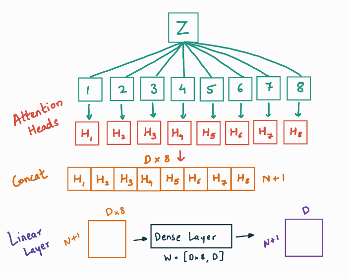
The Scaled Dot-Product Attention as explained above is applied h times (h=8) to get h attention heads. These attention heads are concatenated and passed through a dense Layer to get the final vector of embedded dimension D.
Coming back to our transformer encoder architecture, the Z vector passes through multiple Encoder Blocks to give us the final context vector C.
This MultiHead self-attention can be implemented in Pytorch as below.
Step 3: MLP head
Once, we have our context vector C, we are only interested in the context token c0 for classification purposes. This context token c0 is passed through an MLP head to give us the final probability vector to help predict the class. The MLP head is implemented with one hidden layer and tanh as non-linearity at the pre-training stage and by a single linear layer at the fine-tuning stage.
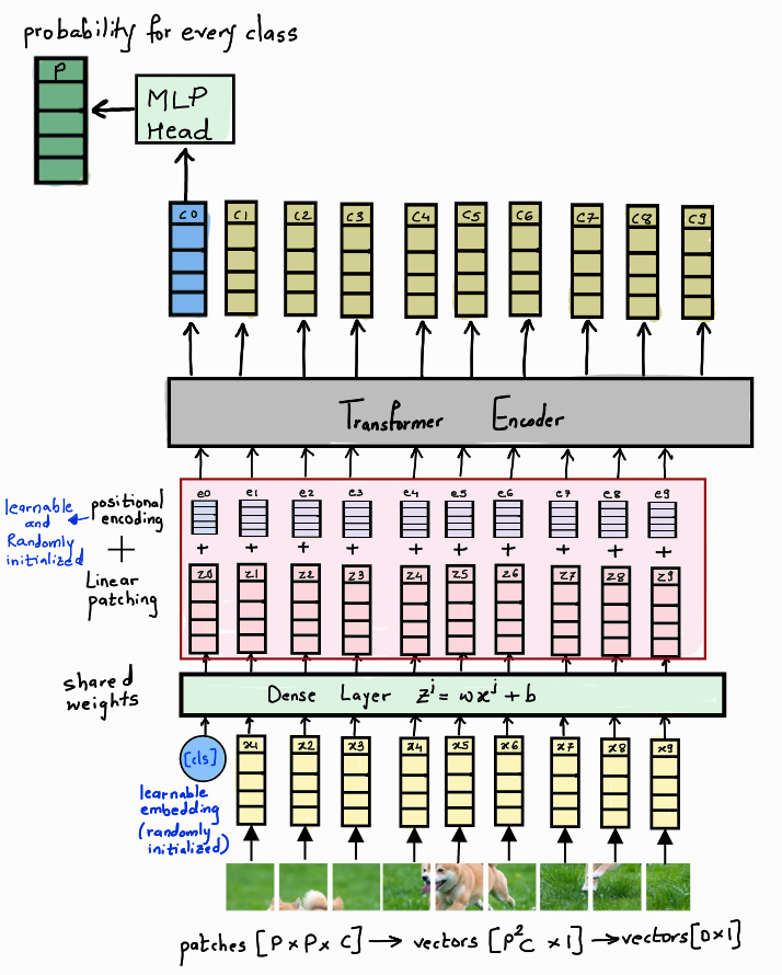
The final architecture is shown in the diagram above. The linear image patches are appended by a [CLS] token and passed through a Dense Layer to get the final encoding vector Z along with positional embeddings. This is then passed through a Transformer encoder architecture to get the context vector C. The value of the context token c0 is passed through an MLP head to get the final prediction.
Here is a PyTorch implementation of the Vision Transformer for reference. It uses the MultiHeadSelfAttention class as implemented above.
For validating our code, we trained our model with MNIST dataset(60k) on a CPU machine for 10 epochs and got an accuracy of 90.85%. For bigger datasets, you may require a GPU machine for training.
Test set: Average loss: 0.9649, Accuracy: 9198/10000 (90.85%)Training:
The training process as mentioned in the paper is divided into pre-training and fine-tuning steps as seen in the below image. For example, the ViT H/16 model is first trained on JFT 300M dataset and then fine-tuned on ImageNet or CIFAR datasets.
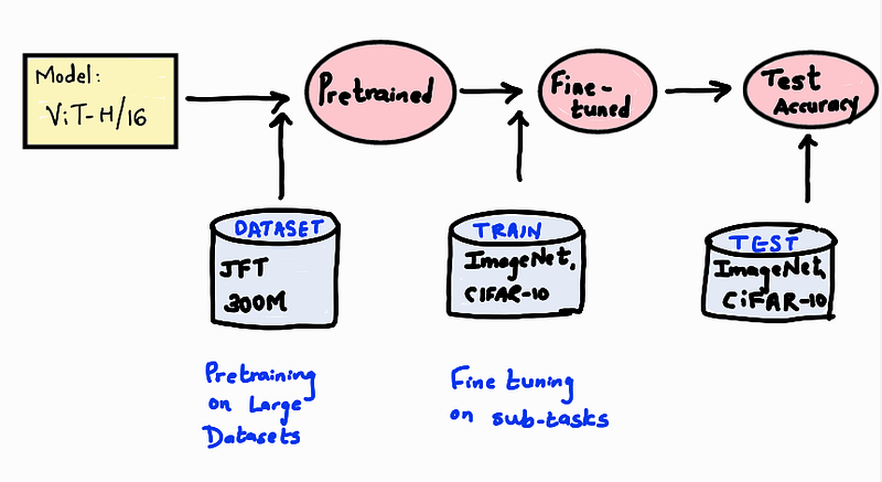
Pre-training:
The network is first pre-trained on a large dataset by randomly initializing the weights. The paper uses 3 pre-training datasets. All 3 models are pretrained with Adam optimizer with batch size of 4096 and weight decay of 0.1.
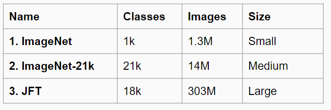
There are 3 main architectures used are as below.
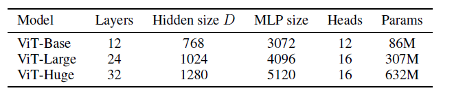
Fine-tuning:
Once the models are pre-trained on large datasets we now fine-tune ViT models on a smaller dataset using SGD with momentum and batch sizes of 512 and 518 for ViT-L/16 and ViT-H/14 models respectively.
Experiments
Scaling Up
To understand the impact of the size of the pre-training dataset on model performance, the authors train Vision transformers on large datasets and compare the results to BiT, trained on the same datasets.
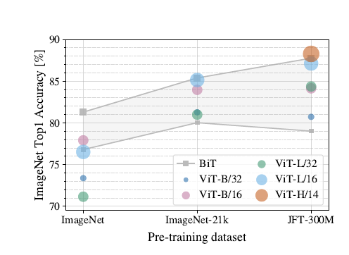
ViT performs significantly worse than the CNN equivalent (BiT) when trained on ImageNet (1M images). However, on ImageNet-21k (14M images) performance is comparable, and on JFT (300M images), ViT outperforms BiT.
Comparison to the state of the art:
We first compare our largest models ViT-H/14 and ViT-L/16 to state-of-the-art CNNs — 1. BiT (Big Transfer) 2. Noisy student.
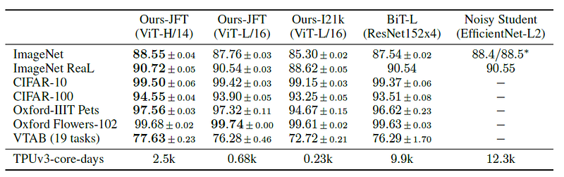
As we can see for ImageNet, the previous state-of-the-art model Noisy Student had an accuracy of 88.4%. The ViT-H/14 outperforms this benchmark while the ViT-L/16 trained on JFT and ImageNet21k performs slightly worse than the benchmark model for the ImageNet dataset.
But for the other benchmark datasets like CIFAR, oxford, and VTAB, the ViT-L/16 and ViT-H/14 models perform better than the state-of-the-art ResNet models while taking fewer resources to train.
As we can see, the number of TPUv3 core days required by the ViT models is considerably less than the BiT and Noisy Student models, which proves that ViT models not only perform well but also train much faster than the existing state-of-the-art models.
ViT also works well on diverse tasks, for example, on the VTAB-1k suite (19 tasks with 1,000 data points each)
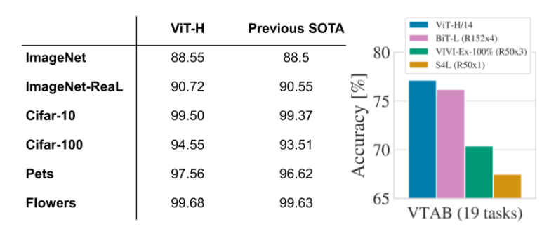
As seen, Vision Transformer matches or outperforms state-of-the-art CNNs on these popular benchmarks as well.
But, why does Vision Transformer perform better?
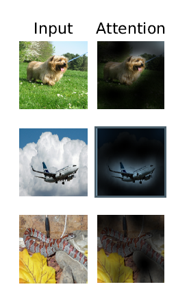
To understand this let us inspect the attention maps in Vision Transformer.
The Multi-Head Attention in Vision Transformers helps it to only pay attention to the relevant part of the image. If we take the average of the output of all the attention heads, we can see this mechanism in action. The model attains to image regions that are semantically relevant for classification.
Transformers are yet not mainstream
Through this simple yet scalable strategy of ViT when coupled with pre-training on large datasets matches or exceeds the state of art on many image classification datasets while being relatively cheap to pre-train the paper sets future scope to analyze the performance of ViTs on other computer vision tasks, such as detection and segmentation.


