CNNs and Vision Transformers: Analysis and Comparison

Exploring the effectiveness of Vision Transformers and Convolutional Neural Networks (CNNs) in image classification tasks.

Image classification is a crucial task in computer vision, widely utilized by companies in diverse fields such as industry, medical imaging, and agriculture. Convolutional neural networks (CNNs) have been a significant breakthrough in this area, and they are used extensively. However, with the advent of the paper “Attention is all you need,” the industry has been shifting towards Transformers. Transformers have demonstrated significant progress in AI and data science. For example, ChatGPT’s impressive performance is a recent illustration of the effectiveness of Transformers. Similarly, the ViT paper provides an overview of Vision Transformers. In this post, I will try to compare the performance of CNNs and ViTs (Vision Transformers) on the Food-101 dataset for image classification. It is essential to note that the choice of using CNNs or ViTs depends on several factors, including the type of work, training time, and computational power, and we cannot directly claim that Transformers are better than CNNs. This analysis aims to provide insights into their performance in this particular task.

Dataset

Due to limited computational power, I partitioned the readily accessible Food-101 dataset, containing approximately 101,000 images, into 10 classes. The dataset can be directly used from PyTorch as well as TensorFlow:

If you want to download the dataset you can use the following link:

https://data.vision.ee.ethz.ch/cvl/datasets_extra/food-101/

I divided the dataset into the following 10 classes:

['samosa','pizza','red_velvet_cake', 'tacos', 'miso_soup', 'onion_rings', 'ramen', 'nachos', 'omelette', 'ice_cream']

Note: Class Names are not in the same order as the above list

The images are transformed and resized to 256x256 and normalized to a mean of 0 and a variance of 1. After the subset of the dataset, the dataset was split into training and validation with the split being 7500 training images and 2500 testing images.

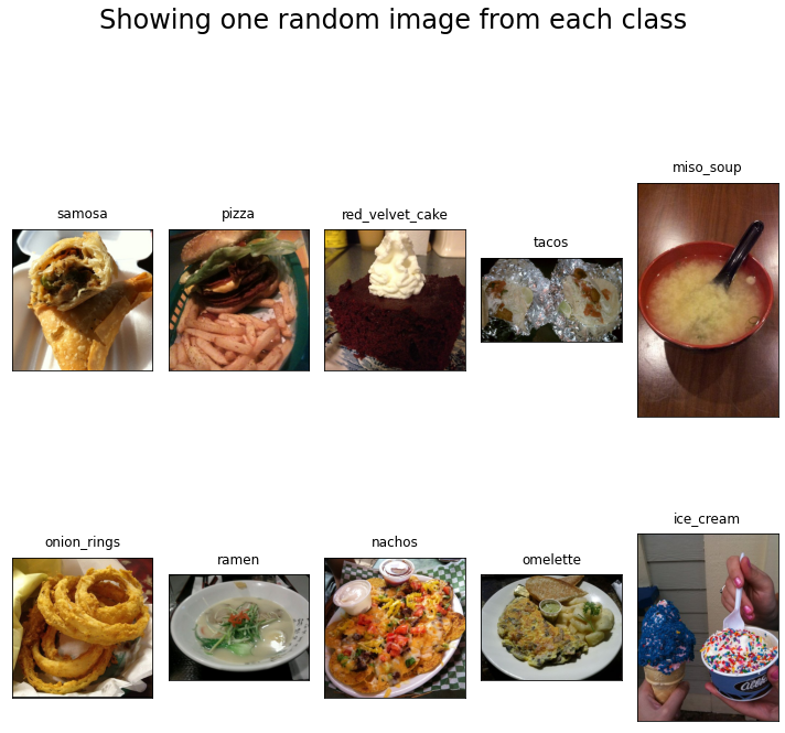
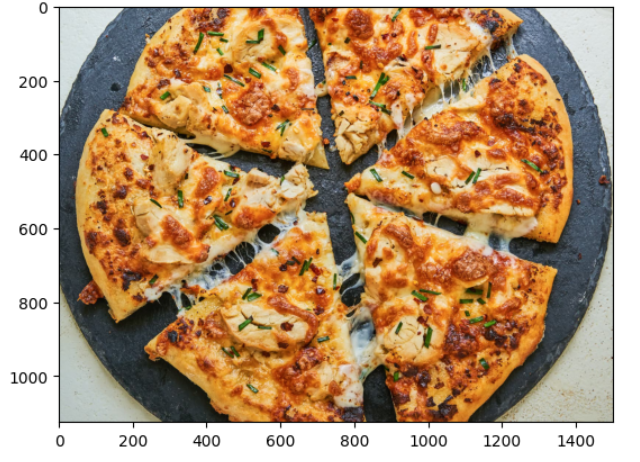
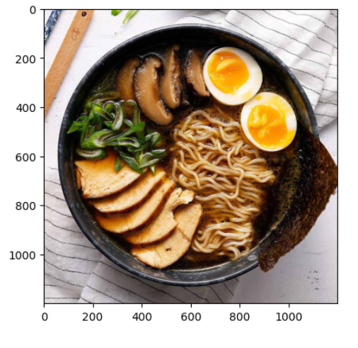
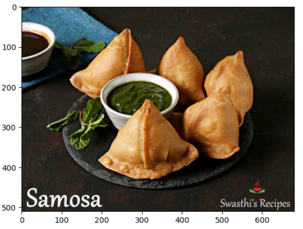
These are the sample images from the dataset:

To compare the performance of CNNs and ViTs, I utilized a pre-trained DenseNet121 architecture for CNNs and ViT-16 for Vision Transformers. The selection of DenseNet121 was based on its dense architecture with 121 layers, making it a suitable candidate for comparison with ViTs in terms of training time, number of layers, and hardware and memory requirements. For ViTs, I used the ViT-Base model, which comprises 12 layers and 86M parameters.

DenseNet121

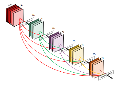
DenseNet-121 is a pretty famous CNN architecture used for image classification and is a part of the DenseNet model family that was designed to address the problem of vanishing gradients that can occur in very deep neural networks. It has 121 layers and uses a combination of Convolutional layers, pooling layers, and fully connected layers. There are 4 dense blocks, each consisting of multiple Conv layers with BatchNorm and ReLU activations. Between the dense blocks, there are transition layers that reduce the spatial dimensions of the feature maps using pooing operation. Here is the architecture of DenseNet —

The pre-trained model was used from PyTorch. The model was trained for 10 epochs.

# Constants
NUM_CLASSES = 10
LEARNING_RATE = 0.001

# Model
densenet = torch.hub.load('pytorch/vision:v0.10.0', 'densenet121', pretrained=True)
for param in densenet.parameters():
  param.requires_grad = False

# Change classifier layer
densenet.classifier = nn.Linear(1024,NUM_CLASSES)

# Loss, Optimizer
criterion = nn.CrossEntropyLoss()
optimizer = optim.Adam(densenet.classifier.parameters(), lr=LEARNING_RATE)

Plots of Accuracy vs Epochs and Loss vs Epochs:

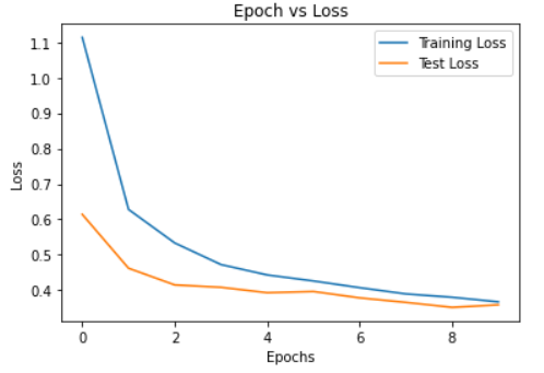
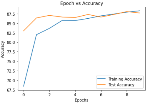
At the final epoch, train loss was 0.3671, test loss was 0.3586, train accuracy was 88.29% and test accuracy was 87.72%.

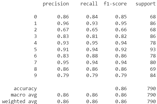
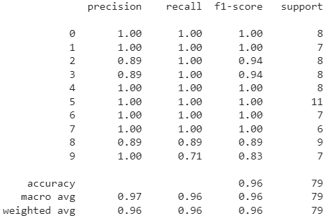
Classification Report:

ViT-16

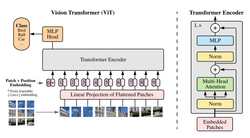
ViT-16 is a variant of the Vision Transformer (ViT), it gained popularity after ViT paper due to its ability to achieve state-of-the-art results on various image classification benchmarks. ViT-16 consists of a transformer encoder, followed by a multi-layer perceptron (MLP) for classification. The transformer encoder is composed of a sequence of 16 identical transformer layers, where each layer contains a self-attention mechanism and a feedforward neural network. The input to the network is a flattened image patch sequence, which is obtained by dividing the input image into non-overlapping patches and flattening each patch into a vector.

The self-attention mechanism in each transformer layer allows the network to focus on different parts of the image when making predictions. In particular, it computes the attention weights for each pair of positions in the input sequence, allowing the network to attend to different patches depending on their relevance to the current classification tasks. The feedforward neural network in each transformer layer then applies a non-linear transformation to the output of the self-attention mechanism.

After the transformer encoder, the output is passed through an MLP classifier, which consists of two fully-connected layers with ReLU activation and a softmax output layer for classification. The MLP takes the output of the final transformer layer as input and maps it to a probability distribution over the output classes.

Following is the architecture of ViT —

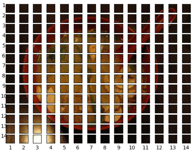
Before feeding the images to the transformer encoder model, we need to first divide the input image into patches and then flatten the patches. Here is an example of the image divided into patches —

Segmented sample input image into patches

I built the transformer model from scratch however the performance was not great. Then I tried transfer learning and used a pre-trained ViT-16 model and default weights from PyTorch. I also applied the transforms on the images suitable for ViT.

# Default weights
pretrained_weights = torchvision.models.ViT_B_16_Weights.DEFAULT

# Model
vit = vit_b_16(weights=pretrained_weights).to(device)

for parameter in vit.parameters():
  parameter.requires_grad=False

# Change last layer
vit.heads = nn.Linear(in_features=768, out_features=10)

# Auto Transforms
vit_transforms = pretrained_weights.transforms()

Plots of Accuracy vs Epochs and Loss vs Epochs:

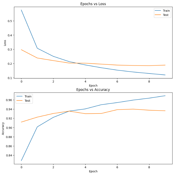
Plots of Accuracy and Loss against Epochs for ViT-16

At the final epoch, train loss was 0.1203, test loss was 0.0.1893, train accuracy was 96.89% and test accuracy was 93.63%.

Classification Report:

Predictions:

Here are some predictions with unseen data for the ViT-16 model —

Note: Class Names are not in the same order as the above list

In most of the cases, ViT-16 was able to classify the unseen data correctly.

Conclusion:

In this specific task, the performance of ViT-16 was found to be superior to that of DenseNet121 in terms of image classification. The accuracy and plot curves also demonstrate a significant difference between the two. The classification report reveals that the f1-score of ViT is better as compared to DenseNet.

However, it is important to note that while Vision Transformers may outperform CNNs in some cases, it cannot be generalized that they are better than CNN architectures. The performance of each architecture is dependent on various factors, such as the use case, data size, training time, parameter tuning, memory, and computational power of the hardware used.

References:

Attention is all you need paper — https://arxiv.org/abs/1706.03762
DenseNet paper — https://arxiv.org/pdf/1608.06993.pdf
Vision Transformers paper- https://arxiv.org/pdf/2010.11929.pdf