Summary

This context is a hands-on tutorial on building a Bayesian Marketing Mix Model using PyMC to measure marketing effectiveness.

Abstract

The context provides a step-by-step guide on building a Bayesian Marketing Mix Model using PyMC. The tutorial starts with a brief introduction to Bayesian regression and its benefits in producing accurate results with less data. The author then uses 2-year media spend and revenue data to model revenue using the Bayesian Marketing Mix Model. The tutorial covers the application of carryover and lag effects, defining saturation functions, adding control variables, and defining priors. The author also demonstrates how to construct the model, evaluate model posteriors, and evaluate model fit. The results are presented in a contribution chart and a table, which are useful in determining the best-performing channels.

Bullet points

The context is a hands-on tutorial on building a Bayesian Marketing Mix Model using PyMC.
Bayesian regression is a way of doing regression analysis that takes into account prior beliefs about the parameters of the model.
The author uses 2-year media spend and revenue data to model revenue using the Bayesian Marketing Mix Model.
The tutorial covers the application of carryover and lag effects, defining saturation functions, adding control variables, and defining priors.
The author demonstrates how to construct the model, evaluate model posteriors, and evaluate model fit.
The results are presented in a contribution chart and a table, which are useful in determining the best-performing channels.

Marketing Mix Modeling: Hands-on with Bayesian MMM using PyMC

Marketing Mix Modeling Series

Part 1: The Art of Measuring Marketing Effectiveness Part 2: 7 Metrics to Use and Boost Your ROI Part 3: Choosing Causal Variables and KPI Part 4: Transform Your Marketing Data with Carryover, Lag, and Saturation Part 5: Strategies to Control Bias in Marketing Mix Models Part 6: Hands-on with Bayesian MMM using PyMC Part 7: Response Curves and Budget Optimization

Thank you for following along my MMM series until this point. Apologies, but the theory was required. Now I will dive into a practical implementation of MMM. And how….in Bayesian style.

As a reminder, Marketing Mix Models are aggregated measurement tools. They attribute revenue to media over longer timeframes — 1 month, 1 quarter or 1 year. If you want to learn about campaign level attribution, check out this article that explains Multi-Touch Attribution with a case study.

Let’s move on and wear our coding shoes.🙃

Bayesian Regression in a nutshell

Bayesian regression is a way of doing regression analysis that takes into account your prior beliefs about the parameters of the model. For example, if you have some reason to believe that the slope of the line is positive, you can use a prior distribution that reflects that. The prior distribution is combined with the data to get a posterior distribution, which is the updated belief about the parameters after seeing the data. The posterior distribution can be used to make predictions, estimate uncertainty, and test hypotheses. Just by incorporating prior knowledge, a Bayesian style regression model can produce accurate results that are in-line with the real world using very little data. As data science begins to solve more complex problems where there is a dearth of data, we are entering into what they call — the era of “Small Data”.

In this post, I will get down to brass tacks and build a Bayesian MMM from scratch.

Media Data

Let’s grab our 2-year media spend and revenue data. If you want to follow along, you can download it here.

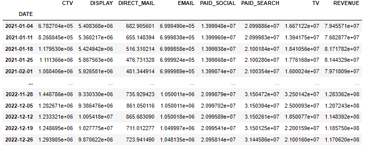
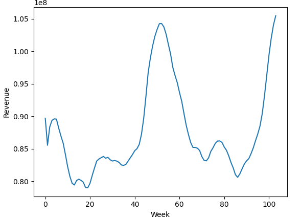
I am going to model Revenue using a Bayesian Marketing Mix Model. If you want to review the other kinds of KPIs that MMM’s model, go here. While time-series forecasting methods decompose a series into trend, seasonality and noise, a MMM decomposes it into media contributions, trend, seasonality and other variables.

Applying Carryover and Lag

If you recall from this post, media effects are retained beyond the day/week in which the ads are run — this is called Carryover. Some channels like TV have a high delay in the effect that the ad has on audience, while Paid Search has an almost immediate effect.

I have individually defined the Lag values for every channel and the retention rate is 0.8. This means 80% of the ad effect is carried over into the next period. Retention length helps control how far ahead the effects can be; typically, this isn’t more than a quarter.

Defining Saturation Function

I will use the Hill function for saturation and it is pretty much the state-of-the-art. It takes two parameters — alpha and gamma — both of which I will fine through Bayesian optimization for every channel. Alpha controls the S-shape of the saturation curve while gamma controls the diminishing effect.

Adding Control Variables

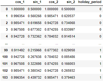
I will add 3 control variables — trend, seasonality, holiday flag. Trend will be added in the model as a lagged value of revenue. Seasonality is modeled through Fourier series of degree 2 — you can revise the formula. The Fourier terms will be min-max scaled because we do not want negative terms in the model except for Trend.

The Holiday flag is set to 1 in the last weeks of the year.

How do we define Priors?

In a Bayesian regression, prior knowledge (or assumptions) is added in two ways — location and distribution. Let me explain the two with examples.

A location-based prior is used to inform the model what the coefficients approximately are. This comes straight from collaborating with marketing teams or through campaign results from publishers like Google or Meta. For example, as you can see in the code we expect Paid Search coefficient to be around 15%.

The second one is a distribution-based prior which is informed by how certain we are of our location-based assumption on the coefficients. It’s defined typically using a Normal distribution with constraints (coefficients cannot be negative for media since contribution should be a positive number). Similarly, I have set prior distributions on the alpha and gamma parameters of Hill function.

Constructing the Model

Let’s stitch it all together into a model. I have mean-normalized the X and Y variables to speed up the Bayesian Optimization and make the coefficients directly interpretable as contributions. This is no different than other modeling algorithms.

All variables are scaled to the magnitude of the KPI, which in this case is revenue. This helps the coefficients be directly interpretable as contributions.

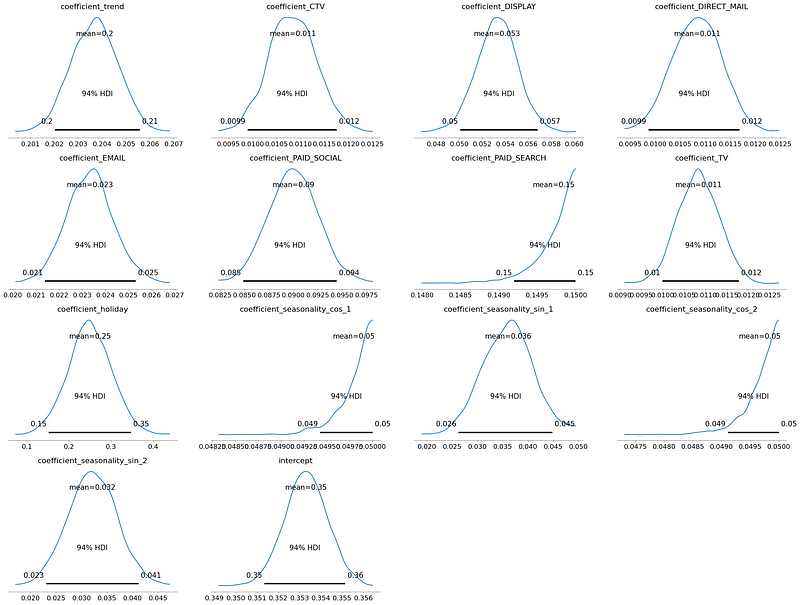
Evaluate Model Posteriors

It’s useful to check the posterior plots. The shape of the plots should match the shape of the prior distribution.

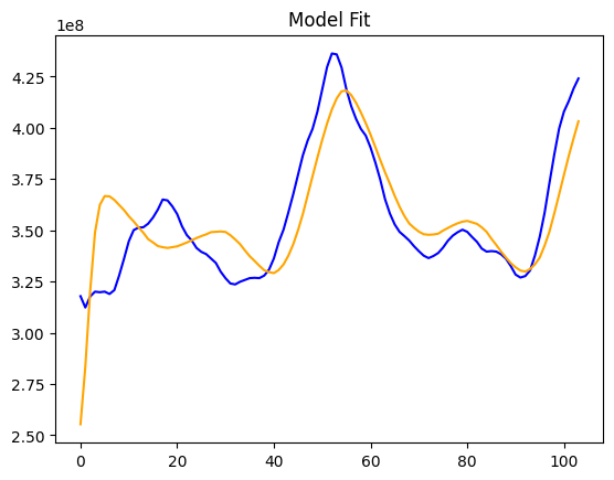
Evaluating Model Fit

There are also traditional methods from regression that are useful in checking model fit. R-squared and MAPE are used most frequently. We can see our model has fit the data well and we have a MAPE of 3.9.

I have also plotted the actual revenues against the Posterior Predictive values. We use the model posterior to generate data that we expect to see, and we check if it matches the data that we actually see. This way, we can make sure that the model is reasonable to describe the observed data.

Results

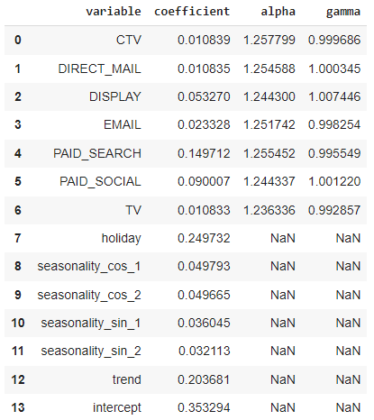
Finally, here’s the results collated into a contribution chart and a table. The coefficients have moved a bit from the priors after observing the data. As you can see, the model is pretty stable and is also learning. Charts like these are useful in determining our best performing channels.

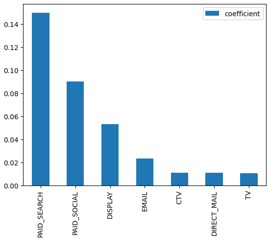
This table has all the information about channels — attribution and saturation.

In the next post, I will use these results to construct response curves. They help us determine how much incremental revenue a change in spend in a channel would bring. All of this was of the past — eventually I will show you how to build an optimizer that will help in planning scenarios based on spend and effectiveness.

Stay tuned!