
Mamba: Can it replace Transformers?
A lot of research effort has gone into making Transformers efficient. Transformers are great, no doubt about that, but they are very resource and data-intensive. Research like Flash Attention, RetNet, and many others show great potential, but somehow Transformer remains the king. In this paper review, we will talk about a completely new architecture called Mamba.
It enjoys fast inference (5× higher throughput than Transformers) and linear scaling in sequence length, and its performance improves on real data up to million-length sequences. Mamba achieves state-of-the-art performance across several modalities such as language, audio, and genomics as a general sequence model backbone. On language modeling, our Mamba-3B model outperforms Transformers of the same size and matches Transformers twice its size in pretraining and downstream evaluation.
Table of Contents
- Understanding Attention memory requirements
- Other methods to solve memory problems
- Why does Mamba look promising?
- Problems with RNN
- What is a “Structured State Space Model” (SSM)?
- Mamba 🐍
- Hardware Acceleration
- A Simplified SSM Architecture
Are you looking for AI content that’s both original and insightful instead of repetitive and copy-pasted content? Want to delve deeper into the technological aspects rather than skimming through surface-level tips and tricks? Discover the AIGuys Digest Newsletter.
And if you want to up your AI game, please check my new book on AI, which covers a lot of AI optimizations and hands-on code:
Understanding Attention memory requirements
The efficacy of self-attention is attributed to its ability to route information densely within a context window, allowing it to model complex data. However, this property brings fundamental drawbacks: an inability to model anything outside of a finite window, and quadratic scaling with respect to the window length.
The big breakthrough in Self-attention was the network's ability to relate different parts of inputs with each other no matter the distance. This importance is directly dependent on the output. For different types of output, the attention given to each token in the input data sequence will vary quite significantly. But the problem lies in scaling this type of system. In order to calculate attention scores, we need to store an NxN matrix of attention scores for a sequence of length N. That means scaling will become more and more resource intensive as we go in the order of context window of 32K.
Note: These attention scores need to be stored in the cache memory or RAM, not in the Hard disk, that’s why it is so hard to train LLMs locally.
To better understand the memory requirement, let’s consider a scenario:
A transformer model like BERT-base, with 110 million parameters; A sequence length of 512 tokens; A hidden size (d) of 768; 12 attention heads; A batch size of 32; Using 32-bit precision.
- Parameter Memory: Each parameter is a 32-bit float, which is 4 bytes. So, the memory for parameters is 110 × 10⁶ × 4 bytes.
- Attention Score Matrix Memory: The size is n² × h × b × 4 bytes (for 32-bit floats). With n = 512, ℎ = 12, and b = 32, this gives the memory required for the attention score matrices.
- Intermediate Matrices Memory: Q, K, and V matrices are each of size n × d × b × 4 bytes. Multiplying by 3 for Q, K, V.
In the given scenario, the total memory requirement is approximately 0.93 GB.
This shows that even for a quite small model memory requirement is a lot, for a system of the scale of GPT, it is tens of thousands of times more, because of quadratic scaling. They even had to make a completely new data center to train such a model with a budget of around 100 million USD just in computing.
Click here to do a complete dive into Self-attention and Transformers.
Other methods to solve memory problems
One very interesting paper I read related to this recently was Flash Attention 2.
How Flash Attention 2 is better?
Flash Attention 2 basically keeps most calculations in the cache or High Bandwidth memory or HBM, but usually, these are very small in size, and it’s impossible to store the entire attention matrix in there.
Solution: Divide the attention matrix into smaller blocks and compute things for them.
This creates another problem, in order to normalize the attention score we need to have the attention values of the entire row.
Solution: A clever way of Normalizing and rescaling
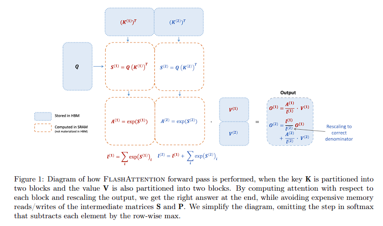
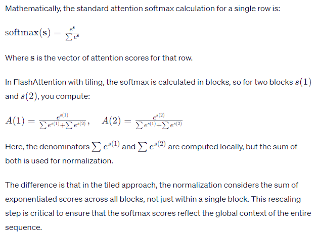
Note: Now this might look like more calculations, but remember they can keep a lot of calculations in HBM and that’s what makes it faster.
Reducing Non-Matrix Multiply Operations: FlashAttention-2 minimizes non-matrix multiply FLOPs (floating point operations per second) which are slower on GPUs due to the lack of specialized compute units for these operations. By focusing on matrix multiplication (matmul) operations, which GPUs can perform more efficiently, FlashAttention-2 aligns better with the hardware capabilities.
Parallelization and Work Partitioning: The algorithm parallelizes the attention computation not just across batch sizes and the number of heads, but also along the sequence length dimension. This enhances GPU resource utilization. Furthermore, within each thread block on the GPU, work is distributed across different warps (groups of threads), reducing the need for shared memory access and improving computational efficiency.
I would highly recommend reading the paper or listening to the author himself: Click here
Other methods with Attention approximation
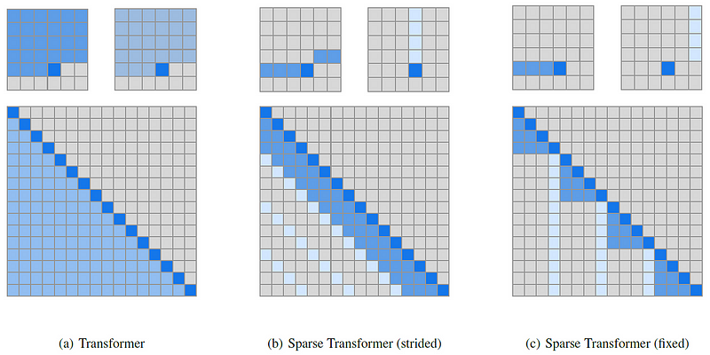
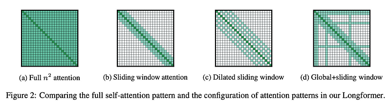
Sparse Attention: Sparse Attention patterns, like the ones used in the Longformer, selectively focus on a subset of the key-value pairs instead of the full set. This can involve attending to a fixed window of surrounding words or implementing patterns that ensure every word still gets a global view periodically, such as diagonal or strided attention. This reduces complexity from quadratic to linear or log-linear with respect to sequence length. Paper: Click here
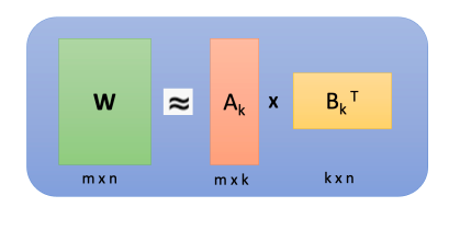
Low-rank Attention: This approach leverages the assumption that the attention matrix can be approximated by a product of two smaller matrices. By reducing the rank of these matrices, you reduce the number of computations required to perform the attention operation. This is effective because, in practice, attention matrices often have low-rank structures where only a few components are significant. Paper: Click here
Kernelized Attention: In models like the Performer, the softmax function is approximated using positive definite kernels. These methods map the original vectors into a Reproducing Kernel Hilbert Space (RKHS) where the attention operation is approximated as a dot product, allowing for an unbiased estimation of the attention mechanism with linear complexity. Paper: Click here
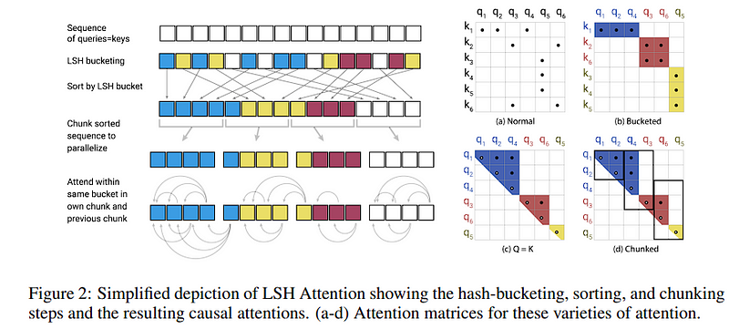
Reformer: It uses locality-sensitive hashing to approximate the dot-product attention. Tokens are sorted into buckets based on hash similarity, and attention is only computed within each bucket. This method is efficient because it reduces the number of comparisons that need to be made. Paper: Click here
Linformer: The Linformer projects the keys and values onto a lower-dimensional space using learned linear projections, which reduces the time and space complexity from quadratic to linear in terms of sequence length. This works well when the attention matrix does not need to capture extremely fine-grained relationships within the data. Paper: Click here
Longformer: The Longformer model uses a sliding window mechanism to limit each token to attend only to nearby tokens, plus a few global tokens that can attend to tokens anywhere in the sequence. This hybrid approach allows for both local and global context to be captured efficiently. Paper: Click here
Why does Mamba look promising?
Mamba achieved a fivefold increase in processing speed over traditional Transformer models, demonstrating linear scalability in relation to sequence length, rather than the typical quadratic. This efficiency extends to sequences with lengths reaching a million elements.
This advancement opens new avenues not only in text-based applications such as conversational AI, summarization, and search, but also in fields like audio synthesis, genomic analysis, and complex time series forecasting, where modeling extensive sequences is crucial.
The name “Mamba” is inspired by its foundation in S4 models, standing for “Selective Structured State Space Sequence Models” — a title as swift and potent as its namesake snake. 🐍
As far as why we need this, it’s already defined in full detail in the above section, the quadratic scaling of the attention score matrix.
To understand Mamba, we need to understand a few more things like the problems with RNN.
Problems with RNN
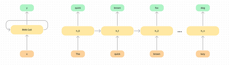
A few years ago RNNs were really popular but there are two main issues with recurrent networks.
- RNNs collapse all the information down to a hidden space and tend to forget information on longer sequences
- RNNs are fast for generation but slow for training
What we mean by “collapse all the information” is imagine trying to save all the information in a sentence into a small hidden space. In the diagram below we can see that the model has to be selective in what it remembers as it goes along.
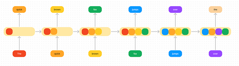
Capturing a comprehensive context within the confined latent space is challenging, particularly when attempting to retain details from both the beginning and end of a sequence.
Historically, GRUs and LSTMs have utilized gating mechanisms in their recurrent cells to judiciously retain or discard information throughout the sequence processing.
However, the capacity of the hidden state to hold context is inherently limited, despite sophisticated gating strategies.
Compounding the limitations of RNNs is their tendency for slow training due to the need for sequential computation, as well as their susceptibility to the “vanishing gradient” problem, where gradients may diminish or become excessively large during backpropagation through long sequences.
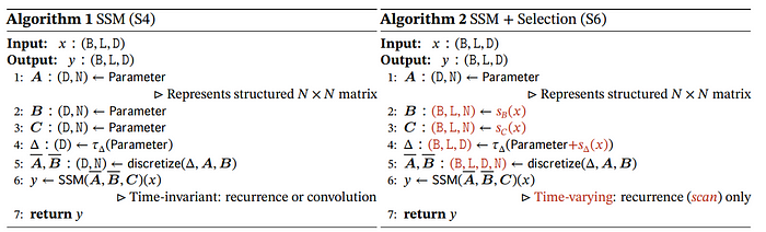
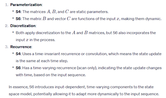
What is a “Structured State Space Model” (SSM)?
SSMs are at the core of Mamba, so it is important to note how they work. We can think of them as the replacement for the self-attention mechanism in a transformer.
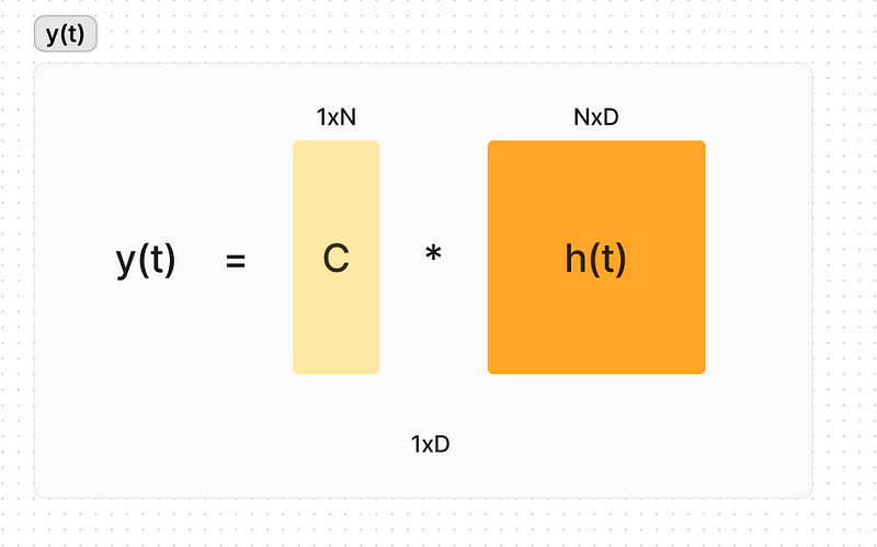
State Space Models (SSMs) offer a structured way to represent and analyze sequences efficiently. In the context of neural networks, an SSM can be used as a layer to process sequences, where the core concept is to map an input signal to a latent state and then to an output signal. The update and output equations for an SSM are:
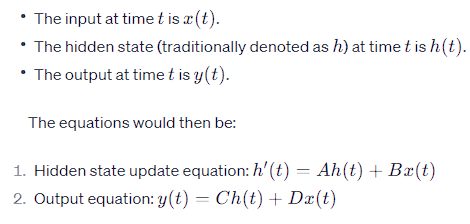
Here, A, B, C, and D are matrices that define the system’s dynamics, with A representing how the state evolves, B how the input influences the state, C how the state is translated to an output, and D a direct feed-through from input to output.
Note that different from your standard recurrent network — it is just fully linear, and does not have the non-linear transforms that a LSTM or GRU have inside them.
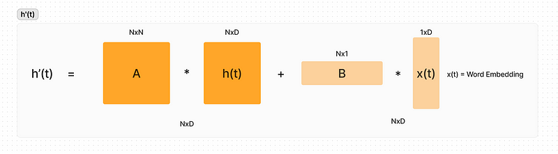
The intuition behind using SSMs in neural networks is to transform the input sequence into a higher-dimensional space (latent state), where its dynamics can be captured more effectively before projecting it down to the desired output. The matrices A, B, and C transform the input data into a latent space that evolves over time, allowing the model to capture temporal dependencies. The discretized version of the SSM makes it computationally feasible to apply this continuous-time concept to discrete-time data, like sequences in machine learning tasks.
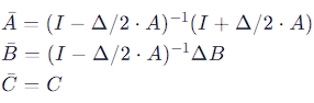
To use SSMs in a discrete setting, such as with neural network training, the model is discretized, often using a method like bilinear transformation, leading to the discrete update equations:
These discrete equations allow the SSM to be applied to input sequences in a manner akin to recurrent neural networks (RNNs), but with the ability to train like convolutional neural networks (CNNs) when unrolled. This approach can significantly improve the efficiency of modeling long sequences.
The bilinear transformation method used in SSM discretization is like deciding how often to take these snapshots and ensuring that important characteristics of the continuous ‘movie’ (like the motion or changes in the scene) are accurately captured in these discrete ‘frames’. The matrices ˉAˉ and ˉBˉ are the tools that help us translate the continuous flow into a series of steps without losing the essence of the process we’re modeling.
Sequence modeling is the art of compressing context into a smaller state, and then using it to predict the output sequence.
Attention does not compress the context at all, it gives the model full access to the history. Attention can be used with RNNs and has been in the past, it is just quite computationally expensive.
There is an efficiency vs effectiveness trade-off of how well models compress their state. If you have a small state with little context, you will be more efficient. If you have a large state with lots of context the model will be slower but more accurate.
Mamba 🐍
Contributions they make in this paper to SSMs are as follows
- A selection mechanism, that allows the model to filter out irrelevant information, and remember relevant information indefinitely.
- A hardware aware algorithm that computes the model recurrently but does not materialize in the expanded state, optimizing for GPU memory layouts.
The combination of these two techniques give the following properties
- High quality results on language and other data with long sequences
- Fast training and inference
- Memory and compute scale linearly in sequence length during training
- Inference involves unrolling the model one element at a time with constant time per step, with no cache of previous elements
- Long context — performance improvements up on real data up to sequence length 1 million
In short, Mamba is the advanced version of S4.
Hardware Acceleration
The model efficiently stores its parameters in SRAM and they perform the discretization and recurrence in SRAM while writing the final outputs to HBM (high bandwidth memory).
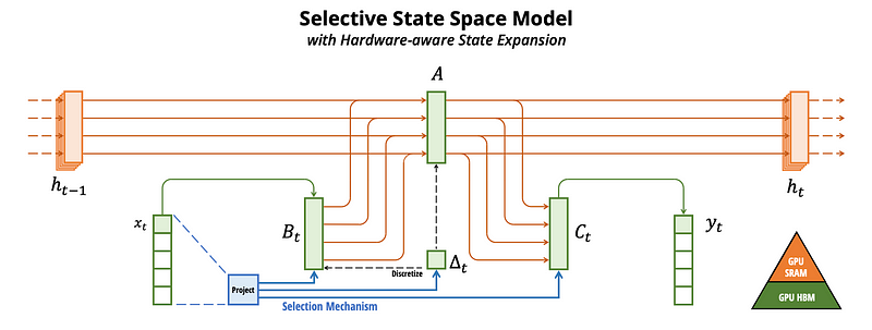
The trick is how you organize the vectors and matrices to minimize copies between memory locations and enable some parallelization during the scan. “With selectivity, SSMs are no-longer equivalent to convolution, but we leverage the parallel associative scan.”
A Simplified SSM Architecture
Selective SSM blocks can be incorporated as standalone transformations into a neural network, just like you would a RNN Cell like an LSTM or GRU. The full architecture of a Mamba block is below, and is not just the SSM module we covered above. There are linear projections, convolutions, and non-linearities surrounding the SSM block in a larger Mamba block.
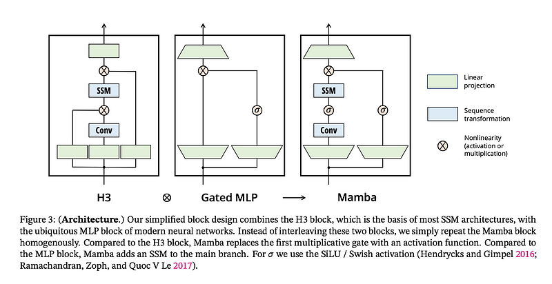
They first project the input up through a linear layer that expands the dimensionality of the input, they also add a residual connection on the right-hand side similar to the transformer.
Then they run a 1D convolution over the linear layer, pass it through a SiLU / Swish activation function, before it gets to the SSM block we talked about above.
The residual path then connects back with the output of the SSM and they shrink the dimensionality back down to the same as the input with a final linear layer.
An important connection: the classical gating mechanism of RNNs is an instance of the selection mechanism for SSMs.
That’s it for today, for results and evaluation I would suggest reading the original paper given in reference.
Writing such articles is very time-consuming; show some love and respect by clapping and sharing the article. Happy learning ❤
Please don’t forget to subscribe to AIGuys Digest Newsletter


