Machine Learning — Understanding data

We will use Titanic data set and try to understand the data

Whenever you start a machine learning project, you will have data from different sources compiled into a single source. Having done that we now need a better understanding of all the features to predict a target variable.

To understand machine learning basic, please refer to my post -https://readmedium.com/machine-learning-demystified-4b41c3a55c99

When we have the target variable available for some of the observations based on historical data and want to predict a target variable then we use supervised learning.

If we do not have the target variable available for observations then we need to use unsupervised learning.

Titanic dataset and data dictionary is available here -https://www.kaggle.com/c/titanic

Python code on Jupyter notebook sued in this post is available at https://github.com/arshren/MachineLearning/blob/master/Machine%20Learning%20step%201%20-%20understanding%20data.ipynb

In our example of Titanic data set, we want to predict if a passenger survived or not.

In the train.csv file we have observations that contain the input features as well as target variable :Survived.

In this post, we will analyze the data in train.csv to identify features helpful to predict if a passenger survived or not.

we will first download the dataset. I have downloaded my dataset in my default jupyter folder

We need to import pandas and numpy libraries

import numpy as np
import pandas as pd

we will now read the data from the downloaded dataset. and we will use the training dataset — train.csv

For more details on how to read data from a different formats of file and how to write to different formats of file follow my post— https://readmedium.com/python-reading-and-writing-data-from-files-d3b70441416e

data_set = pd.read_csv("train.csv")

let’s see what are the different features we have in the titanic dataset by printing a small subset of the dataset. Here we are printing first three rows only.

data_set.head(3)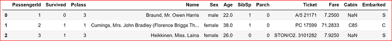

we need to find out the no. of columns in the dataset, no. rows in the dataset what are the data types for each column and for that we will use info() method.

data_set.info()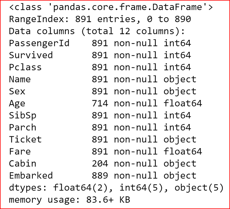

From the output above we know that we have null values for Age, Cabin and Embarked columns as the row count in the dataset is 891 and these columns have not null value count less than 891

we can generate the descriptive statistics that summarizes central tendency including Nan values.

To know more about descriptive statistics refer to my post -https://readmedium.com/descriptive-statistics-bc01594c4cbe

If the datatype is numeric then output will contain count, mean, std, max, min, and 25%, 50% and 75% data

If the datatype is object then we will see count, unique, top and freq.

we can also show the statistics for all the features in the data set

data_set.describe(include='all')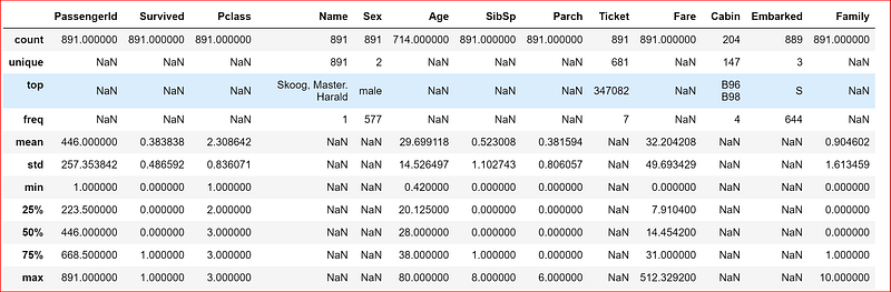

since our data set has numeric and objects let’s display the descriptive statistics

First we will take all the numeric features and display their statistics

data_set.iloc[:,[0,1,2,5,6,7,9]].describe()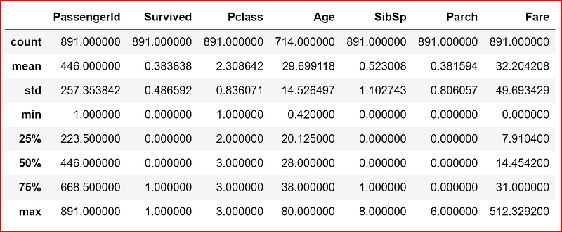

we now let’s display the statistics about the features with object data type using either of the one statement

data_set.iloc[:,[3,4,8,10,11]].describe()

data_set.describe(include=['O'])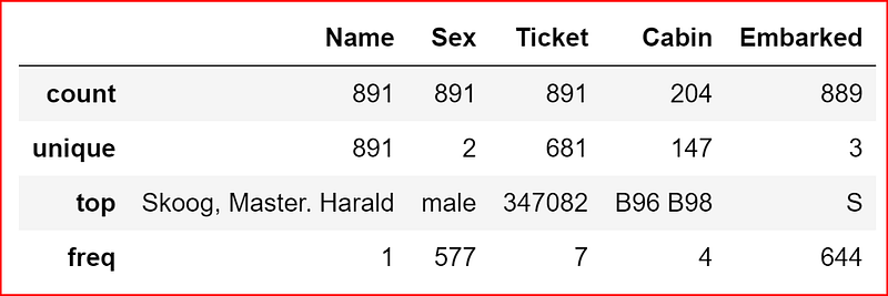

once we understand the data we can check for correlation between different features .

Before going into correlation let us see if we can do any feature engineering on the data set using our common knowledge. In real world, it will be based on our domain knowledge

when we look at the data dictionary we see that column SibSp is # of siblings or spouses on board and Parch is # of parents or children on board. based on common understanding or in machine learning language based on feature engineering we can combine these two columns and call that as family as sibling and spouses forms our family.

Here we have used the Dictionary feature to sum values from two columns and assign it to a new column added to the data. Detailed explaination is available in my post -https://readmedium.com/python-data-structures-dictionary-9b746b94b421

data_set["Family"] = data_set["SibSp"] + data_set["Parch"]
data_set.head(3)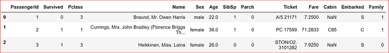

Now diving into correlation

What is correlation?

Correlation is when a change in one variable may result a change in another variable

Correlation coefficients range from -1 to +1

Correlation coefficient of +1 signifies perfect positive relationship. For a positive increase in one variable there is a positive increase in second variable

Correlation coefficient of -1 signifies perfect negative relationship, the two variables move in opposite directions. For a positive increase in one variable there is a decrease in the second variable

Correlation coefficient of 0 means there is no relationship between the two variables.

We will use corr() method to get the correlation of all features in our data set

data_set.corr()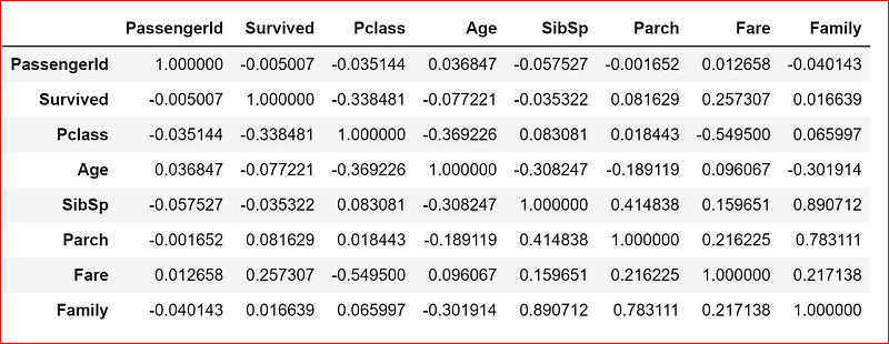

what do we interpret from these numbers?

In this data set we will analyze the correlation coefficient of all features with respect to the Survived feature. This will helps us understand if a feature has an impact on the passenger’s survival chance.

Based on the correlation data above we make the following deductions

1. Passenger Id does not have a significant impact on passenger’s survival due to a value close to 0 between PassengerId and Survived feature
2. Pclass has a negative correlation with survival means a third class passenger has a low survival chance
3. Age has a negative correlation with Survival. Higher the age lower the survival chance
4. Siblings and Spouses seems to be have a negative correlation with survival chance
5. Parents and child have a positive correlation with survival chance
6. when we combine spouse, sibling, parents and child as Family, we see a slight positive correlation with Survival chance
7. Fare has a positive correlation. A first class passenger had a higher chance of survival compared to a third class passenger based on the fare. Here we assumed that the first class passenger paid a higher fare compared to a third class passenger.

In Machine Learning, we need to remove all assumption and base everything on facts.

Let’s verify our hypothesis by querying the data for all passenger who paid fare more $100 and checking if the Pclass is 1

data_set[data_set['Fare'] >100]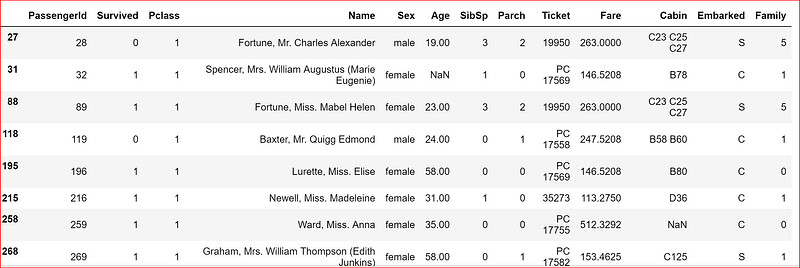

Let’s check what was the average fare paid by third class passenger

np.mean(data_set.loc[data_set['Pclass'] ==3, 'Fare'])

13.675550101832997

That proves our understanding of the data.

To get a deeper and better understanding of the data efficiently we should visualize the data.

For Data Visualization refer to my POST