
Simple Linear Regression in Python
Step-by-step follow along | Data Series | Episode 4.3

From the previous two episodes you should now know the underlying theory of Linear Regression, its purpose and how we use gradient descent in optimising our parameters. You can read them here: Episode 4.1, Episode 4.2 .
You can view the code used in this Episode here: SampleCode
Setting up your programming environment
All programming in this series will take place on a program called Anaconda which is the most popular data science toolkit for performing machine learning tasks in Python and R.

You can download Anaconda completely free by visiting https://www.anaconda.com/products/individual
After downloading Anaconda, launch Jupyter Notebook. All our projects will take place on Jupyter Notebook which is a program that enables us to run code on our browser quickly and efficiently.
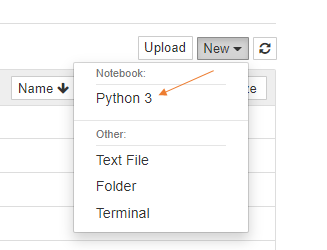
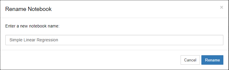
Rename the notebook to Simple Linear Regression by clicking on Untitled.
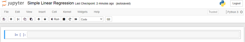
Your environment should now look like this and we are ready to get going.
Importing our Data
The first step of any Data Science project is to import our data into Python. To do so first need to download our data from the following link: Data
Click on “code” and download ZIP.
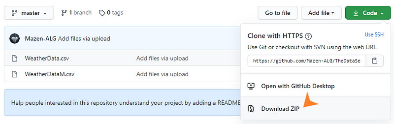
Once the ZIP file is downloaded, open it and locate WeatherData.csv.
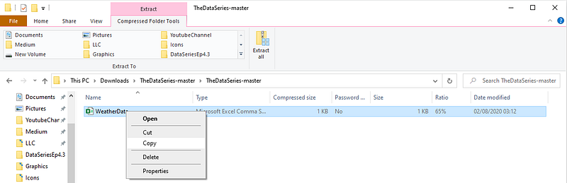
Copy this WeatherData.csv file into your local disk. I would advise creating a new folder called ProjectData to store your WeatherData in.
Note: Keep this medium post on a split screen so you can read and implement the code yourself.
The first step is to import our data into python.
We do that with the following code, make sure you are in Jupyter Notebook:
# Import Pandas Library, used for data manipulation
# Import matplotlib, used to plot our data
# Import nump for mathemtical operations

import pandas as pd
import matplotlib.pyplot as plt
import numpy as np

# Import our WeatherData and store it in the variable weather_data
weather_data = pd.read_csv("D:\ProjectData\WeatherData.csv")
# Display the data in the notebook
weather_data
“D:\ProjectData\WeatherData.csv” | This shows the file path as to where we stored our WeatherData.csv which we downloaded in the previous step. It is important this is correct.
After running the code it should look something like this:
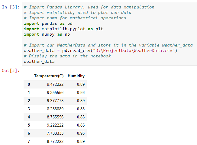
We can see all 50 Temperature and Humidity values.
Plotting our Data
In order to see if linear regression is appropriate for our data we need to plot it and see if follows a linear trend. We do this with the following code:
# Set x to our input Temperature
x = weather_data['Temperature(C)']
# Set y to our output humidity, this is the value we trying to predict
y = weather_data['Humidity']

# Plot Humidity against Temperature
plt.scatter(x, y)
# Add labels to the graph
plt.xlabel('Temperature(C)')
plt.ylabel('Humidity')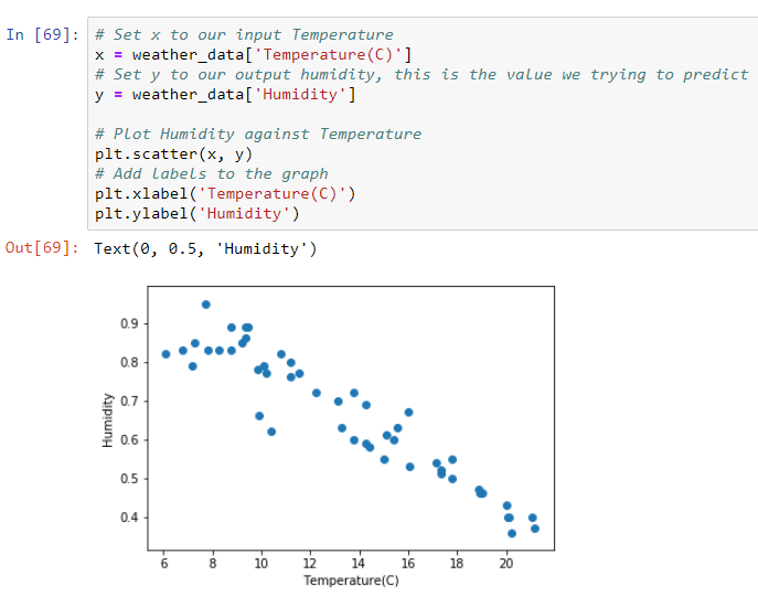
We see our data follows a roughly linear trend and applying linear regression is suitable.
Implementing Simple Linear Regression
In episode 4.1 we gave all the maths needed to calculate a regression line. Thankfully, we can call a function that can do all this maths for us. We call this function from the library sci-kit learn which provides many useful machine learning models like linear regression.
from sklearn.linear_model import LinearRegression

# Setting x and y to the appropriate variables, we reshape x to turn it from a 1D array to a 2D array, ready to be used in our model.
x = weather_data['Temperature(C)'].values.reshape(-1,1)
y = weather_data['Humidity']

# Define the variable lr_model as our linear regression model
lr_model = LinearRegression()
# Fit our linear regression model to our data, we are essentially finding θ₀ and θ₁ in our regression line: ŷ = θ₀ + θ₁𝑥. Gradient descent and other methods are used for this.
lr_model.fit(x, y)
# Find predicted values for all x values by applying ŷᵢ = θ₀ + θ₁𝑥ᵢ
y_pred = lr_model.predict(x)
plt.scatter(x, y)
plt.xlabel('Temperature(C)')
plt.ylabel('Humidity'

# Here we are plotting our regression line ŷ = θ₀ + θ₁𝑥
plt.plot(x, y_pred)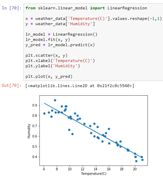
We can find θ₀ and θ₁ by implementing the following code:
theta_0 = lr_model.intercept_
theta_1 = lr_model.coef_
theta_0, theta_1
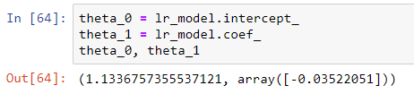
Here we discover θ₀ to be 1.13.. and θ₁ as -0.035 which matches the regression line we calculated in Episode 4.1.
Using our regression model to make predictions
The purpose of calculating our regression line in the first place is to use it to make predictions. In this case, if we were given a new temperature value what humidity value can we roughly expect to get?
# input 32 into our regression model "np.array([32]).reshape(1, 1)" reshapes 32 into a 2D array. This is done as our model only accepts inputs of this form.
y_pred = lr_model.predict(np.array([32]).reshape(1, 1))
y_pred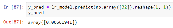
So based on our regression line a temperature value of 32°C expects to give us a humidity of around 0.0066, which seems reasonable looking back at our temperate vs humidity graph we plotted earlier.
Side note:
You may have noticed a lot of reshaping of data going on which seems quite unnecessary, however sci-kit models are built to only accept inputs in a certain format. Converting a number like we did above into a 2D array essentially makes the following conversion:
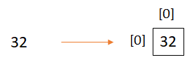
Putting 32 in the position (0,0) of a 2D array.
Another way to convert 32 into a 2D array is by using the following [[32]].


