How to Create a Pivot Table with Python/Pandas in a Jupyter Notebook

Translating one of Excel’s most useful tools into Python/Pandas

A pivot table is an incredibly useful tool for organizing a large set of data into a statistical summary of that same data set.

But you probably already know this. You are here because you’d like to learn how to translate one of your favorite techniques for summarizing data in an Excel workbook into a Jupyter Notebook. Let’s dive in.

Table of Contents:

1. Set up your notebook
2. Grab some CSV data from Kaggle
3. CSV to Dataframe
4. Pivot Table, and Playing with the Pivot Table

Step 1: Setting up your notebook

This tutorial assumes a little familiarity with Jupyter and Python. If you are just getting started, start with my tutorial here:

If you already have Jupyter, Python, and Pandas installed then don’t go anywhere!

Setup is easy. We’ll need pandas, and we’ll need numpy for the type of pivot table we will be doing. Numpy will be helping us calculate the aggregation type (count of values).

import pandas as pd
import numpy as np

Honestly. It’s really that simple.

Note: If you get an import error, it’s probably because you haven’t added the package to your environment, or activated your environment. Head over to your Anaconda Navigator and make sure to add the package needed to whatever environment you activate for your Jupyter Notebook work. Apply the update, and don’t forget to restart your terminal before starting up your Jupyter Notebook again!

Step 2: Grab some CSV data from Kaggle

Since we’re replicating one of our favorite features from an Excel workbook, I think it makes a ton of sense to go find a CSV somewhere on the internet, download it to our local machine, and then transform that data into a Dataframe in our notebook.

First, let’s go grab some data. Kaggle.com has plenty of datasets available for us to play with, but you WILL need an account. That’s ok though. It’s worth signing up to access the data, and maybe in the future you’ll be interested in participating in some Kaggle challenges!

I’ve decided to grab data from a dataset called “Movies on Netflix, Prime Video, Hulu and Disney+”

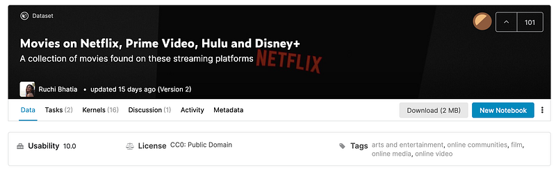
Just hit “Download” to grab a zip file containing the CSV. Then unzip the file. Why am I telling you this? You know what to do!

Step 3: CSV to Dataframe

Now that you have an interesting CSV on your local machine, we’ll import that data into our notebook as a Pandas Dataframe.

The basic command is this:

df = pd.read_csv('')

A cool little trick is hitting the “tab” button after writing: pd.read_csv('~/Desktop')

By hitting “tab” the notebook is smart enough to fill in the full path, and then you can get some auto-complete help like you would in a sticky search bar. See it in action below:

See how the notebook automatically fills in the path ‘/Users/davidallen/Desktop/’? All you have to do is start with ‘~/Desktop’, hit “tab” and the notebook is smart enough to create the full path for you. Neat.

Then you can use the tab trick again for some autocomplete help. Just start writing the beginning of the file name, and then hit the tab button again.

You could also just do the tilda (~) without hitting tab if you want:

df = pd.read_csv('~/Desktop/MoviesOnStreamingPlatforms_updated.csv')

This will work too.

Great. Moving on to the main event: the pivot table!

Step 4: Pivot Table, and Playing with the Pivot Table

Now for the meat and potatoes of our tutorial. We’ll use the pivot_table() method on our dataframe. Our command will begin something like this:

pivot_table = df.pivot_table()

It’s important to develop the skill of reading documentation. So let us head over to the pandas pivot table documentation here.

A pivot table has the following parameters:

.pivot_table(data, values=None, index=None, columns=None, aggfunc='mean', fill_value=None, margins=False, dropna=True, margins_name='All', observed=False

We don’t necessarily need to pass all of these parameters explicitly when we create our pivot table. Pandas will make some assumptions if we leave ignore parameters.

The very basics that we need to set are:

• index
• values
• aggfunc

And it’s also useful to understand that we can structure our pivot table command in two ways.

(1) like this:

pd.pivot_table(df, index='', values='', aggfunc='')

or (2) like this:

df.pivot_table(index='', values='', aggfunc='')

I prefer the df.pivot_table way. Where you call the method on your dataframe. It’s just the way I like to do things.

Anyways…

For this exercise, we are just going to organize all of the data by year. I’m curious how many titles from each year there are on these streaming platforms.

Let’s first take a look at the first 5 rows with the head() method:

df.head()

This returns:

This is nice because we can easily see the names of the columns and all the accompanying data. Now for our pivot_table. We’ll just look at a count of movies from each year:

df.pivot_table(
     index='Year',
     values='IMDb',
     aggfunc=np.count_nonzero
)

You see, this is why we had to import numpy. We needed numpy’s count_nonzero method.

Our result:

I like to flatten out the columns with reset_index() like so:

df.pivot_table(
     index='Year',
     values='IMDb',
     aggfunc=np.count_nonzero
).reset_index()

This gives us a cleaner table by resetting the index and moving the former index, “Year”, to a column of data:

Next, let’s actually assign this table to a variable name, and then rename our columns to be more clear about what data is included in the columns:

pivot_table = df.pivot_table(
     index='Year',
     values='IMDb',
     aggfunc=np.count_nonzero
).reset_index()

And then, rename the columns:

pivot_table.columns = ['Year','Count_of_movies']

Walah:

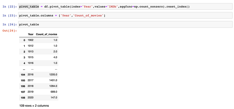
The 2nd column name actually makes sense now.

Next, let’s look at just the last 10 years of data:

pivot_table[-10:]

Looks like 2017 was a popular year for movies!

We could have just as easily looked at the first 10 years of data by doing:

pivot_table[:10]

Next, let’s sort the pivot table by ‘Count_of_movies”. It’ll be interesting to see which years produced the most streaming content. We’ll just look at the top 10 results:

pivot_table.sort_values('Count_of_movies',ascending=False)[:10]

The results:

2017 is indeed our most prolific year so far for streaming content being added to these platforms.

Next, I’m curious which year contains the highest average IMDb rating. Let’s change our aggregation function to np.mean to accomplish this:

mean_pivot_table = df.pivot_table(
    index='Year',
    values='IMDb',
    aggfunc=np.mean).reset_index()

Then let’s update the column names again:

mean_pivot_table.columns = ['Year','avg_IMDB_rating']

And we’ll sort the values by the average rating, looking at just the top 10:

mean_pivot_table.sort_values('avg_IMDB_rating',ascending=False)[:10]

The results:

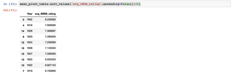
It’s not really surprising that these older movies are better rated. They are only on these platforms because they are popular. The more recent years have plenty of bad ratings alongside the good ratings to bring those averages down.

But I’m really much more curious to learn which year in the 21st century have the best-reviewed movies. Let’s filter out all years except the 2000’s and beyond…

To do this, let’s create a copy of our pivot_table dataframe with a filter:

filtered_pivot = pivot_table.loc[pivot_table.Year >= 2000]

and then sort by rating:

filtered_mean_pivot.sort_values('avg_IMDB_rating',ascending=False)

Note: if you don’t explicitly pass ascending=False pandas will assume ascending=True .

The result:

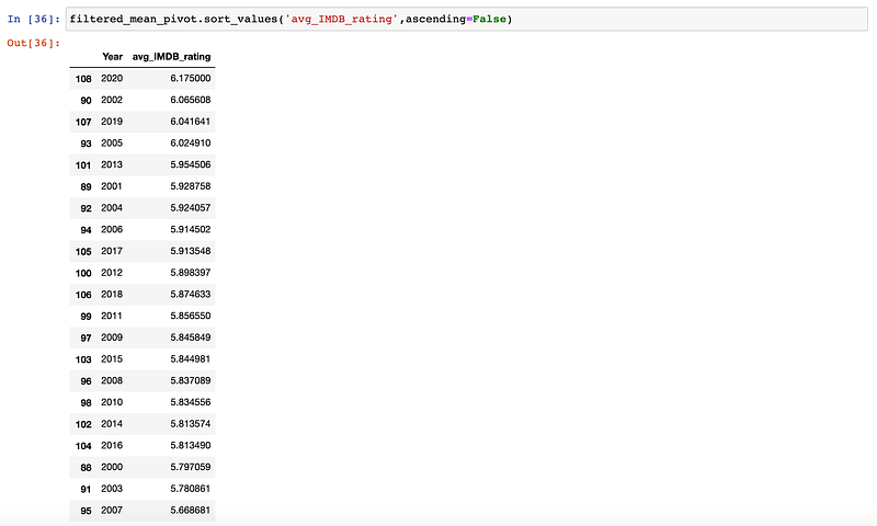
2020 was a good year for movies!

But I don’t think this tells the whole story. Let’s add a new column to this pivot table that will tell us how many movies are included for each year. I have a suspicion that 2020 is the highest-rated year in the 2000’s because only a small number of well-regarded movies have been added to these streaming platforms thus far.

We’ll add our new column by using a method very similar to a vlookup. It’s called map() If you are curious to learn more about vlookups in Python/Pandas, you can learn more in my tutorial here. Onward!

This is the command that will do the business:

filtered_mean_pivot['count'] = filtered_mean_pivot.Year.map(
   pivot_table.set_index('Year').Count_of_movies)

Business done. Let’s look at the results, sorted by IMDb rating, of course:

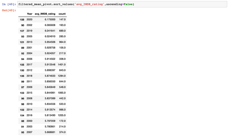
How interesting. Truly.

That’s it for now, folks! I hope you enjoyed this tutorial and learned something useful. Now go get out there and understand the World a little better through your analysis of data! I’m so proud of you and your new-found skills.

If you enjoyed this tutorial, please give it a “clap” or two, share it with your friends, and go ahead and please give me a follow on Medium and Twitter. Your engagement keeps me motivated to keep creating!!

Till next time…

If you enjoy reading stories like these and want to support me as a writer, consider signing up to become a Medium member. It’s $5 a month, giving you unlimited access to thousands of Python guides and Data science articles. If you sign up using my link, I’ll earn a small commission with no extra cost to you.